Since Excel has an extensive number of features, functions, and tools, mastering Excel can seem like a long way road.
When you have a lot of things to grasp at once, it can slow down your performance—be it during data entry, data analysis, creating a visualization, or sheet formatting.
But, what if I tell you there’s a way to become an Excel Ninja pretty fast?
Today, I will share 25 tips (from my experience) to help you save time at work and boost productivity skills.
Use Keyboard Shortcuts
One thing every Excel user should definitely learn is the Keyboard Shortcuts. Excel has over 200 keyboard shortcuts for Ribbons, Workbooks, Selection, and many more that’ll improve your work speed.
So, make a habit of using these shortcuts instead of using the mouse all the time.
It’ll be a game-changer. Trust me!

Also, if you cannot keep tabs on the default shortcuts, you can always create your custom.
I have also written a detailed article on How to Create Your Own Excel Shortcuts.
Use FlashFill and AutoFill
For data entries, Excel’s FlashFill and AutoFill are by far the quickest ways to input values. These are smart, automated tools that pretty much do all your work for you—in a flash.
While these two features may seem similar, there’s actually a difference between them.
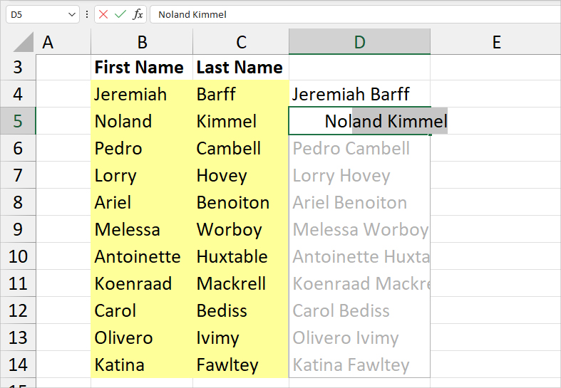
Use FlashFill when you need to fill in the worksheet cells in the same pattern.
For example, if you need to join two columns, just enter the data. When Excel recognizes a pattern, FlashFill will automatically suggest the remaining values to fill. All you need to do is enter Ctrl + E or press Enter.
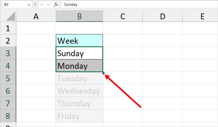
Next, you can opt for AutoFill when you need to copy down the formula or enter a series of values like dates, weekdays, numbers, etc. The most amazing part is you can even create a Custom Autofill.
To use it, hover over the bottom right corner of the selected cell. Then, once you see the cursor, extend the Plus cursor right or down as required.
I recommend this trick to beginners who take hours to type the data one by one.
Create a Drop-Down List
I’ve always loved creating a drop-down list for my data in Excel. Whether it’s to build printable forms, questionnaires, or for dynamic lookup values.
Instead of typing answers for each question, you can have lists of options to choose from.
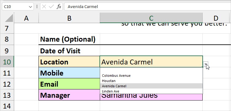
In addition to that, it’s best if you master how to insert a dependent drop-down list. You can set pre-defined options for the main options.

Use Analyze Data
If you use Office 365, this is a plus point as it is only available in this version.
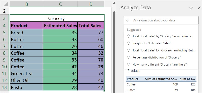
Excel has another automated tool called “Analyze Data,” which suggests suitable Charts and Pivot Tables for your dataset using AI.
Since you do not have to look for the right figure and construct a chart from scratch, it saves a lot of time to create a data visualization.
You could even find the suggestions to create Charts based on criteria in the Analyze Data menu. Simply click on Insert PivotChart or Insert Chart to use it.
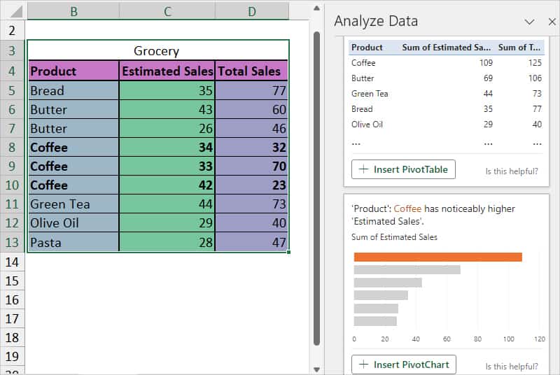
Similarly, the next notable feature of this tool is that you can ask for insights about your data like the Percentage distribution of ‘Grocery.’
Freeze Panes
For data entry or data analysis, you may find the need to keep certain parts visible. Rather than scrolling through up and down or sideways, you can Freeze Panes to lock it.
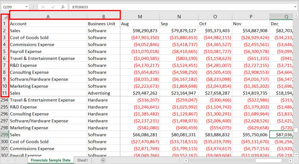
You could freeze the top row and first column only or freeze multiple columns and rows at once.
Once you’re done, you can unfreeze the panes on your sheet.
Hide/Unhide Sheets
If you struggle with managing the number of worksheets on your Excel file, learn how to hide or Unhide Sheets.
After you hide the unwanted sheets, referencing and switching in between sheets will become a lot earlier.
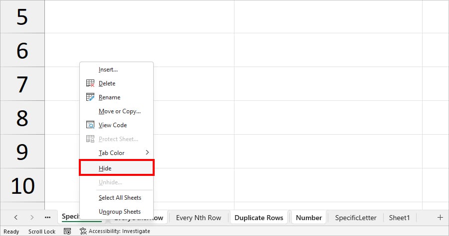
Moreover, this also saves you from transferring the data to another sheet as there’s a VeryHidden feature for confidential information.
After you complete your work, you can unhide the sheet.
Casing Functions (UPPER, LOWER, PROPER)
Since some Excel functions are case-sensitive, you might need to format the text strings in the Upper case, lower case, or First letter capital.
As there are no built-in Change case buttons, many users tend to do it manually. But, there are casing functions like UPPER, LOWER, and PROPER to convert text cases.
Use any one of these functions as required.
| Function | Syntax | Use |
| UPPER | =UPPER(text) | Convert text into all capital letters. |
| LOWER | =LOWER(text) | Convert text into all lower letters |
| PROPER | =PROPER(text) | Format text as the first letter capitalized and remaining in the rest lowercase. |

Use TRIM Function
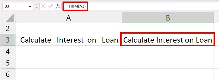
Spaces in Excel can be hard to detect. When a text has extra spaces, it can misguide the formula and result in the wrong outcome. Especially, when you’re counting and extracting characters.
To avoid such a mistake, use the TRIM function to clear spaces. Removing spaces is also a good practice to keep your sheet clean.
Use RAND and RANDBETWEEN Functions
Do you ever find the need to create a mock-up data in Excel?
It can take hours when you think and type in the numbers one after another. Instead, use functions like RAND and RANDBETWEEN to prepare dummy data in seconds.
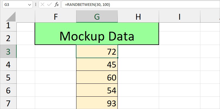
However, you do need to keep in mind that these functions are “Volatile.” It means that when you recalculate the worksheet each time, the formula will automatically refresh and result in new numbers.
To avoid this, copy and paste the generated numbers as values only.
Set Print Area
For users who have to print a certain area of the worksheet repetitively, I recommend you set the Print Area.
With this, you’ll automatically have the same ranges ready on the print page every time you enter Ctrl + P shortcut. So no more wasting time selecting the same cell ranges to print.
We have a detailed article covering several ways to set and format the print area.
Use Stock/Currencies/Geographies Data Type
Excel can recognize the entered texts as a stock, currency, or geographies. So, from the Data tab, use any one of these for your data analysis.
When you change your values into Stocks or Geography, Excel will immediately link them to the online source. Therefore, you can directly import statistical information for that data.
For Instance, if I enter France and click on Geography, Excel displays the overall data about it online.
It includes population, GDP, Leaders, infant mortality rate, and many more. When I click the Field and select an option, it imports values in the cell.
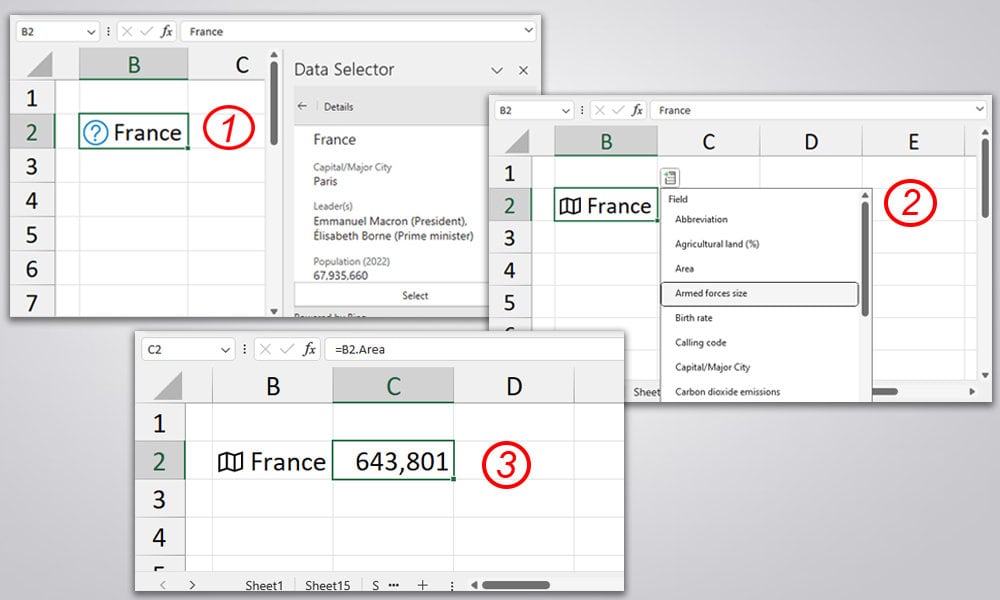
Since you do now have to look for information separately on websites, this will definitely spare you time.
However, the only con is that this feature is limited to only premium users (Excel 365) at the moment.
Use Text to Columns Feature
When importing a file into Excel, there are chances that the worksheet is unorganized, cluttered, and dirty. Most importantly, you might have some jumbled-up texts in the same column.
Either way, if you need to split the information into different columns, Text to Columns is the best tool for it. Why?
Because the tool has the option to separate the columns based on a delimiter and it’s easy to use.
For example, it could be texts with commas, dashes, spaces, etc.
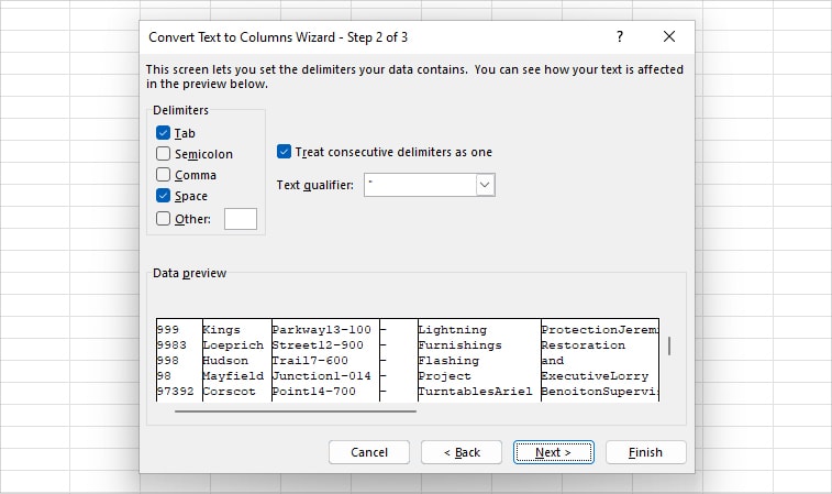
Other than truncating texts in Excel, you can use it to separate names, dates, addresses, date and time, etc.
Paste Special
We all use the Paste Special menu to paste only the specific items or exclude a certain format.
But, Excel’s Paste Special menu can do more than just paste the copied items. It has extra hidden features like Operation and Transpose.
Using the Paste Special menu, you could easily swap the rows and columns. All you need to do is tick the Transpose option in the Paste Special dialogue box and hit OK.
Next, it might sound surprising to most beginners, but you could also add, subtract, multiply, and divide the copied numbers while pasting them.
For example, there are numbers from cell A1:A9. I have copied number 2 in cell C2. Let’s add all the numbers in the column by 2.
For that, I’ll select and right-click on the A1:A9 range, and choose Paste Special. Then, select Add and hit OK. I’ll have the sum without even using any functions.
Isn’t it cool?
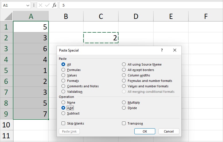
It is a very simple yet faster way to perform calculations for a smaller dataset in Excel.
Turn on Filter
When you have more than thousands of rows and columns, you won’t have time to compare and analyze the data based on criteria.
To make your data evaluation more efficient, try adding the Filter tool.
Display only the required items from the table like “values begins with XYZ” and hide the remaining. This way, you can concentrate on specific information and work on them.
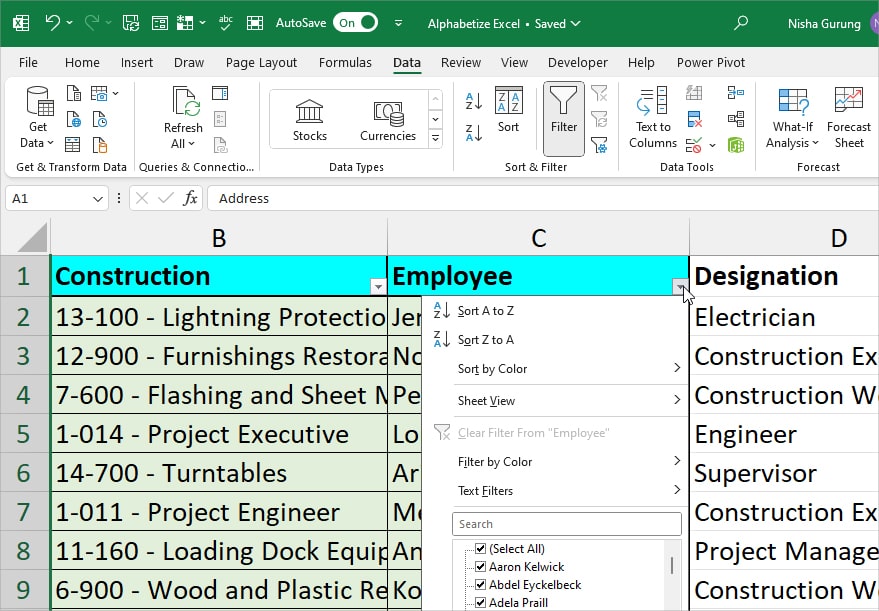
You can use it to delete filtered rows, copy filtered data, etc. There’s even a FILTER function to filter and return items.
Also, for faster performance, I recommend you try these Filter shortcuts in Excel.
Conditional Formatting
Believe me! Conditional Formatting will be your Best Friend when working in Excel.
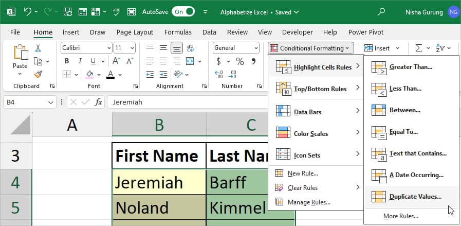
This is because it shades the cells in certain criteria and also allows you to construct your own condition.
Conditional Formatting is one of the best ways to segregate items in a sheet. Just by looking at the highlighted color, you can easily identify the Duplicates, Dates, greater or less than values, specific rows, etc.
It’s also helpful to highlight active rows in Excel. So, isn’t it a time saver?
Create a Data Entry Form
Excel’s Data Entry Form is without a doubt the secret sauce for every data entry geek.
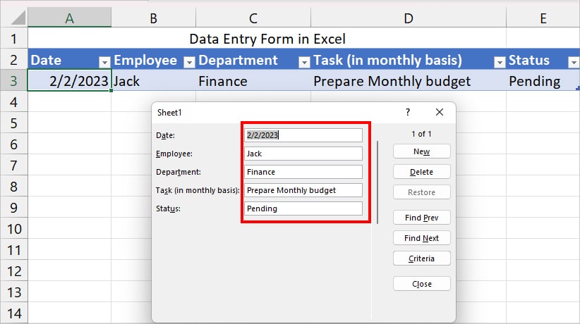
Using a Data Entry form, you could record data of the whole row together, also without any errors.
This applies to a big dataset, too, since it supports 32 columns simultaneously.
Use Data from Picture
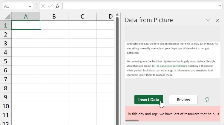
Not many users are aware of this. But, there’s a Data from Picture tool in Excel that allows you to directly load the information from a picture spreadsheet data.
Yes, I can just take a screenshot of a paragraph on the web. Then, using this tool, I can convert and load texts into the Excel Cell. I literally saved myself from typing the online information manually.
This tip might be your Knight in the Shining Armour too.
Use Lookup Functions
When you have a master sheet or multiple worksheets, you may find the need to draw out values from another source. I wouldn’t imagine scanning data manually, locating it, and entering it on the current sheet.
To do that, my go-to method is using Excel’s lookup functions like VLOOKUP, XLOOKUP, HLOOKUP, INDEX and MATCH, OFFSET, INDIRECT, etc.
Although these functions are advanced, they can help you pull out the data from the referenced sheet in no time.
What I like most about using lookup functions is you can make them dynamic by inserting a drop-down list. It’s a big time saver for our daily tasks.
Create and Run Macro
If you use Excel daily and need to perform repetitive tasks like me, record Macro. For me, learning how to create Macros has been—hands down—my biggest turning point in Excel.
It spares you a lot of time as you could just run the record Macros over and over again to automate the tasks.
The best part is Macro can record every task you usually perform like cell formats, data entry, use of Excel Ribbons, each Mouse click, file import, and many more.
It stores all of these actions as the Visual Basic Analysis (VBA) code.
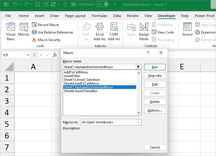
At first, creating Macros or dealing with VBAs may intimidate most beginners. But, you do not have to have the technical knowledge to run macros – unless you need to edit the code.
These are the beginner-advanced-level articles that’ll help you with using Macros in Excel.
- How to Enable Macros in Excel
- How to Create Macros in Excel
- How to Copy Macros in Excel
- How to Modify Macros in Excel
- How to Unblock Macros in Excel
- How to Create Macro Buttons in Excel
- How to Change the Window Size in a Macro in Excel
- How to Use Macro To Delete Rows Based on Criteria
Create Custom Menu/Add to Quick Acess Toolbar
For a more personalized experience, Excel allows its users to customize some of its features.
You can insert your own custom menu in the Ribbon Tabs to easily access it.
For Instance, I have added the Superscripts menu in my New Tab, Ring Alarm in my View Tab, etc.

Similarly, for the menus you use daily, you could load them to the Quick Access Toolbar. This way, you can use the feature with just a single click.

The less you spend time navigating through the menu, the more efficient you will be!
Load Add-Ins
Although there could be several workarounds to do things in Excel, sometimes, using Add-ins could be just the right option.
You’ll have more extended functionality to insert custom ribbons and functions, interact with Excel data, and many more.
For example, if you need to prepare Descriptive Statistics, the ToolPak Add-In would be more faster and effective. You wouldn’t have to calculate all the required values one by one.
Similarly, for What-If Analysis, you could use Solver.
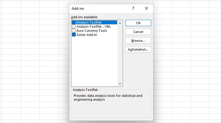
Just like that, load the Excel Add-Ins and take advantage of extra features to enhance your output.
Use Power Query
As the name implies, Excel’s Power Query is the most powerful tool used to combine and transform data. Personally, I use it to import multiple files and merge them into one from different sources.
Power Query involves four phases – Connect, Transform, Combine, and Load.
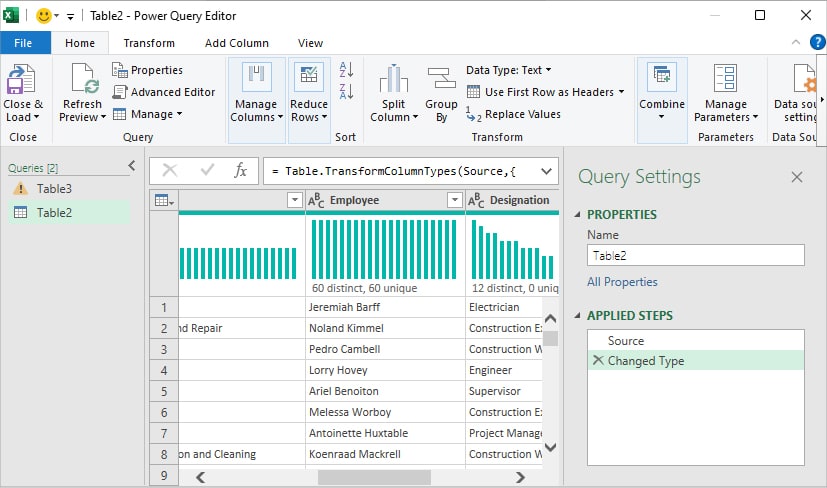
Let’s briefly see each of these phases in detail to know how Power Query would be a big time saver in Excel.
- Connect: You can connect with databases like Web, Azure, Power BI, File, Online Services, etc. Then, import external data from these sources into your Excel.
For Instance, import XML files, TXT files, JSON files, PDF files, POWER BI data, etc. - Transform: In the data transformation, you can modify your raw data. Here, you can Remove duplicates, Group Data, Split cells, Delete Rows/Columns, Replace Values, Sort Data, Switch Rows and Columns, Extract Texts, Count Rows, Count Unique and Distinct Values, do Conditional Sum, Statistics, and many more.
Also, note that you can use all these features to the existing data of your current worksheet. Meaning that you do not have to necessarily import from external sources. - Combine: Next, the Power Query is also best for merging files from different sources. For Instance, combine multiple text files into one, merge queries to combine tables in Excel, join two columns, combine texts, and so on.
- Load: Once you’re done shaping your database, load them into your spreadsheet. However, for users who imported files, you can also skip the transformation part and directly load the data.
Add Pivot Table
Excel’s Pivot Table is one of the perfect tools to summarize and evaluate data. It calculates the sum of identical values and illustrates trends and patterns.
You can add PivotTable for your present worksheet or external data sources.
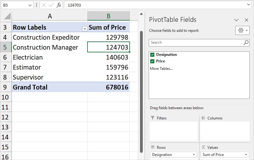
What makes it more incredible is you can refresh a Pivot Table after updating every value. Since Pivot Tables are dynamic in nature, you do not have to insert a new Pivot Table.
Pivot Table also comes with a bonus feature called “Slicer” to filter items in the range. So, filtering data by single or multiple criteria isn’t a big deal. It can come in handy when you are creating a Dashboard in Excel.
To explore more about the Slicer, you can go through “How to Use Slicers in Excel.”
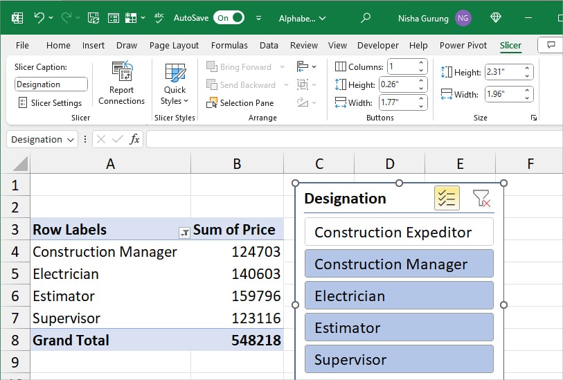
In case you do not want the Pivot Table later, you have the option to Unpivot data i.e. to change it back to the normal Table range.
Consolidate Data
Similar to the Pivot Table, Consolidating data is also another way to create a summary of the information. But, this method is kind of different from what we’ve learned above.
Consolidating data is mostly used to merge the ranges of different worksheets into one. Or, in practical terms, we can also reference it as “Creating a Master Sheet.”
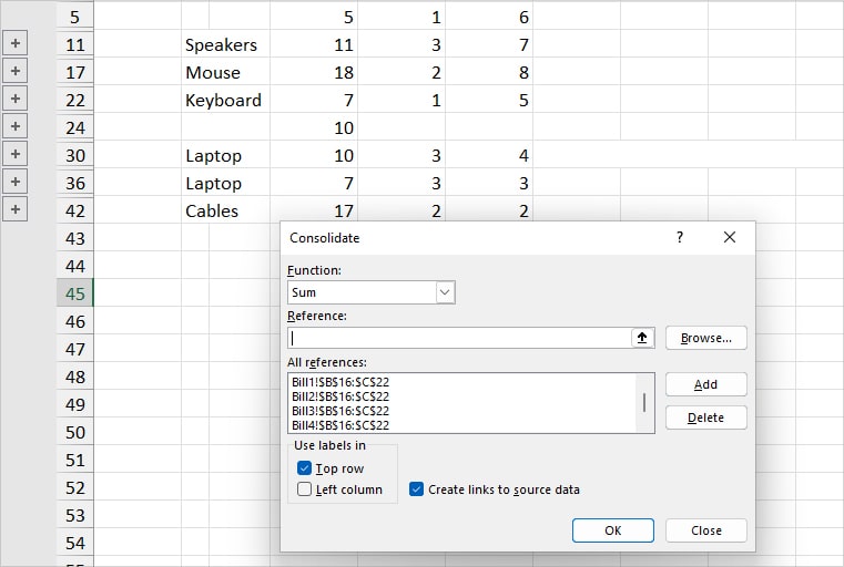
To do this, there is a Consolidate Tool and functions like SUMIF and SUM.
So, if you’re copying and pasting sheet data to find out the aggregate, stop right away!
Use Binary File Format
Having a larger Excel file means laggy performance and taking hours to send/download files, or it could get even worse when Excel keeps crashing.
If you want to have an uninterrupted experience, save the workbooks in the binary file format.
Since it takes less space, it provides you with a faster loading experience. Eventually, you can save time.
Similarly, you could check out our comparison article on XLSB vs XLSM to deep-dive into why this is the best file format.