Excel has hundreds of built-in functions, making it the best tool to perform any calculations. To calculate mass multiplication, you don’t have to go through trials and tribulations to get results.
Personally, I often use multiplication in excel. Whether I’m tracking my monthly budget, calculating my finances, or creating charts and graphs. I prefer the PRODUCT and SUMPRODUCT functions to achieve accurate outcomes within a moment.
As a beginner, however, you can utilize the asterisk arithmetic operator (*) to multiply two given numbers. This gets the job done but is the most basic and tedious formula.
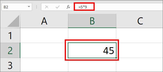
Example: to multiply 5 and 9, enter =5*9 in the cell. You will get 45 as result.
= (number 1*number 2)
Using (*) Asterisk Arithmetic Operator
Case 1: Multiply Columns with Relative Cell Reference
Rather than manually typing each numbers, you can refer to a cell. Here, we will apply the same formula as above but take data from another cell. We will add the Relative cell reference of each column to multiply.
Example: To multiply Column A and Column B in this example., we will use the =A2*B2 formula. The formula arguments will be,
- A2: First cell of Column A to multiply.
- B2: First cell of Column B to multiply.
- Launch Excel and open your worksheet.
- On cell C2, type
=A2*B2and enter. You will get the result.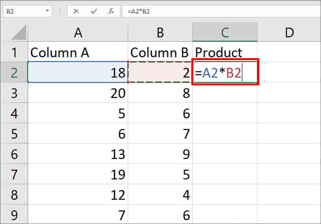
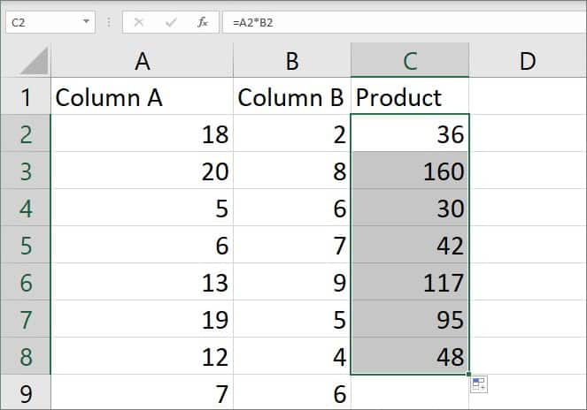
- Now, select the C2 cell and hover over the Bottom-right corner of the cell. When a plus sign appears, drag the cursor down to auto-fill.
After getting the result, you can also use the flash fill to copy down the formula to other cell ranges.
Case 2 – Multiply Columns by Absolute Value
In some cases, you would have to multiply the whole columns of numbers with a single constant number.
Example: multiply all numbers of Column A by the number 5 of Column B.
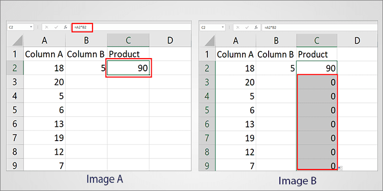
In this case, if you multiply the A2 cell by B2 . i.e. (=18 * 5 = 90), we will get an accurate outcome like Image A. But, when you flash fill to other cells, you will get 0 as shown in Image B.
This is because as per the given formula, cell A3 will multiply cell B3 which has no value (=20* 0 = 0).
To solve this, we will lock the B2 cell by adding dollar signs, making it an Absolute cell reference. Now, your formula will be =A2 * $B$2. So, each cell in Column A will refer to the value of $B$2 for multiplication. The formula arguments are:
- A2: Cell reference to multiply in Column A.
- $B$2: Select the cell with a constant number of Column B. Then, add the $ sign before B and 2.
- On your Excel spreadsheet, click on C2 cell.
- Type a formula
=A2 * $B$2and press Enter.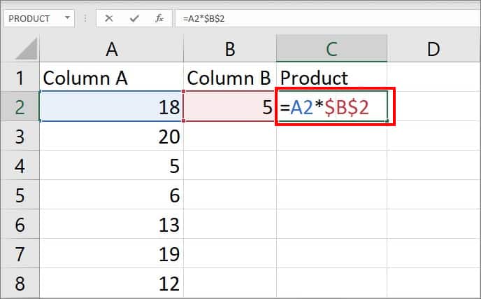
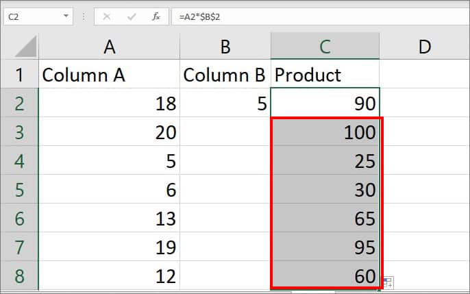
- You will get output in C2 cell. Click on the cell and drag the Plus Icon from the bottom of the cell. It will automatically apply a formula to other cells.
Using PRODUCT function
Above two methods are great when you are multiplying a limited number. But what if your record is in the millions and you need to multiply hundreds of numbers all at once?
For mass multiplication in Excel, you can use the PRODUCT function. This function allows you to multiply about 255 numbers. Let’s check out its syntax and arguments first.
Syntax : =PRODUCT(number 1, [number 2],….)
Arguments:
- number 1: First number you want to multiply. (Required)
- number 2: Extra number you want to multiply. It is optional.
Now, you can go through these two cases with the PRODUCT function.
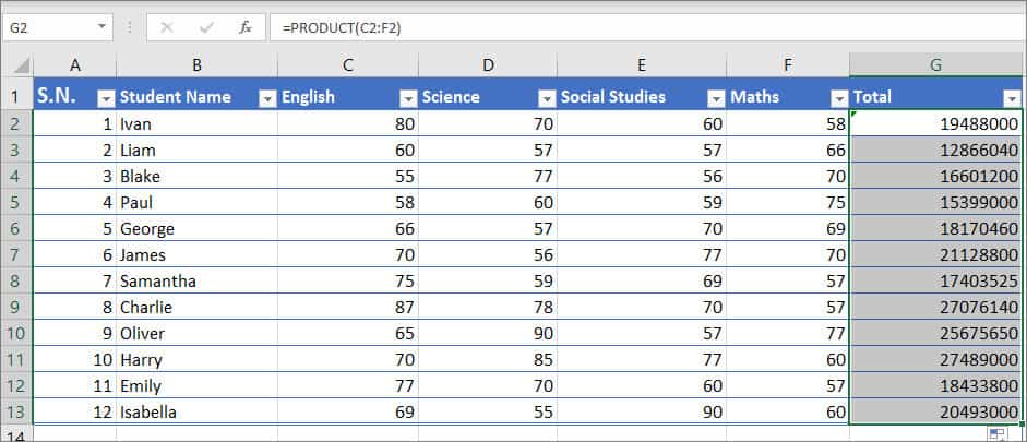
Case 1: Multiply Cell Ranges of a Row
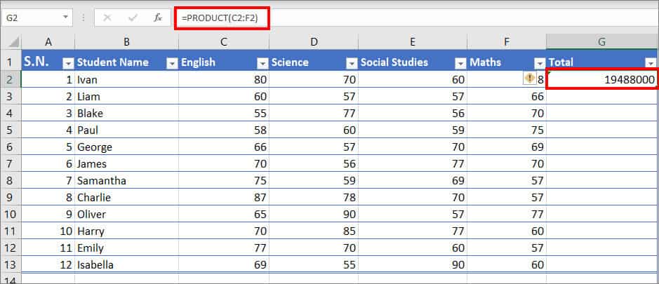
In the given example, suppose you have to multiply the series of cell ranges from C2 to F2. You would have to enter the =C2* D2* E2* F2 with the basic formula. It can be tiring to enter each cell one by one till the last end cell. You might as well enter the wrong cell reference in between.
In such case, the PRODUCT function can make the multiplication process more simplified. To multiply the cell ranges from C2 to F2, we will use the =PRODUCT(C2:F2) formula.
After you get the results, you can use the Auto-fill handle to apply the same formula to other ranges.
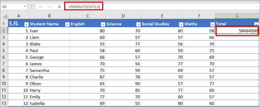
Case 2: Multiply Cell Ranges by Another Number
You can also use the PRODUCT function to multiply the cell ranges of a row first. Then, simultaneously multiply the end result by a number.
In this example, let’s assume, you want to multiply cell ranges from C2 to F2 times number 3. For this, you’d have to enter the =PRODUCT(C2:F2, 3) formula in the Total cell.
Using SUMPRODUCT Function
For complex calculations involving a lot of data, the SUMPRODUCT() Function can be very helpful. People often prefer this method when performing calculations like weighted average, sales analysis, conditional sum, extracting substrings, etc.
Syntax: =SUMPRODUCT(array1, [array 2], [array 3],…)
Arguments for this function are:
- Array 1: Values you want to multiply and sum.
- [Array 2] [Array 3]: Extra values from 2 to 255 to multiply and sum.
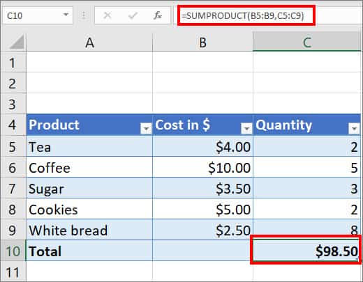
Example: Let’s assume, you need to multiply the cell range of Column B by Column C and add the results. For this, we will use =SUMPRODUCT(B5:B9, C5:C9) formula. This formula will multiply cell B5 with C5, B6 with C6, and so on then add results.
How to Multiply by Percentage in Excel?
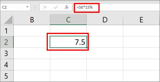
You can use the basic formula. i.e. =number *% to multiply the number by a percentage.
For example, =50*15%. You will get 7.5 as an outcome.
But, if you have to Decrease or Increase the number by a percentage, you’d have to use a different formula.
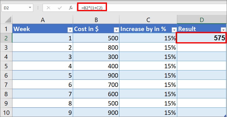
Let’s take a look at the given example to Increase the amount of Column B by a percentage.
Insert the formula, =B2*(1+C2) in D2 cell.
The formula Arguments are:
- B2: First cell of column B with an amount.
- 1: 100%
- C2: First cell of column C with percentage to increase value.
In formula, we have placed (1+C2) inside the parentheses because we want Excel to calculate them first. As per the table, the formula will add (1+0.15 = 1.15) and multiply the results ( 1.15 * 500 = 575). You can drag down the auto-fill handle to copy the formula for other ranges too.
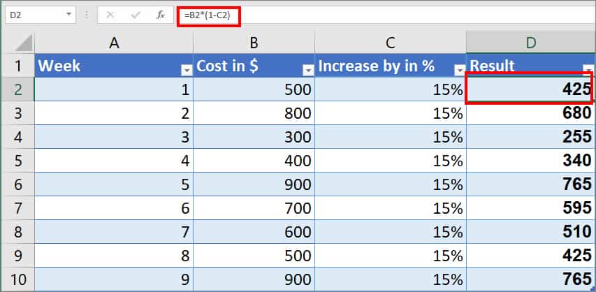
Similarly, in case you want to Decrease the number by a percentage, use =B2*(1-C2)formula.