In Excel, duplicate items aren’t much of a big deal if you’re using them to calculate subtotals. In fact, you can count duplicates to find out the total number of sales, regular customers, and many more.
But, if the duplicate contents are superfluous, it’s pointless to keep them. Such values will only expand your spreadsheet size and make it harder for you to pinpoint the information. Besides, redundant items can also confuse you when using a formula.
So, your best bet is to de-duplicate the values and keep your sheet clean.
Use Remove Duplicates
Excel has a default Remove Duplicates menu to eliminate duplicate values from your range. Remember, since the effect will apply to your data itself, consider creating a backup copy first.
- On your sheet, select the Range.
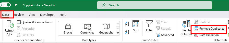
- Go to Data Tab. In the Data Tools section, click on Remove Duplicates.
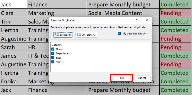
- On the window, tick the Columns you wish to filter duplicate values from and hit OK.
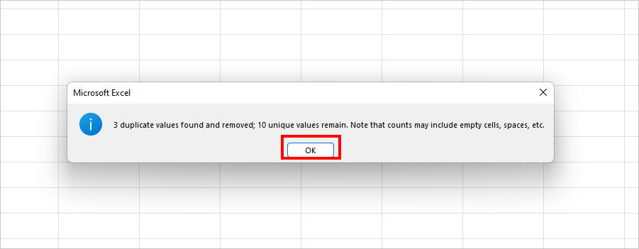
- Again, Click OK.
Use Conditional Formatting
If you’re a regular Excel user, you must be familiar with the Conditional Formatting tool. The Conditional Formatting also has a default highlight cell rule based on Duplicate Values. So, let us use this to shade cells and filter out the duplicate values from the data range.
While you can use Conditional formatting within the same sheet, it is especially more helpful for users who have duplicate values across two different Excel Sheets. Besides, it also comes in handy if you just want to identify the duplicates and not delete them.
Example: Take for instance, you have two workbooks named File 1 and File 2. File 1 has a list of Company Data entries. File 2 contains a few data entries from File 1. Now, if you need to remove the duplicate values in File 1, we will use Conditional Formatting to achieve this.
Although we’ve given the steps to de-duplicate values based on two sheets, the steps are similar for a single sheet too. You can just skip the copy-paste and highlight-pasted content part.
Step 1: Apply Conditional Formatting
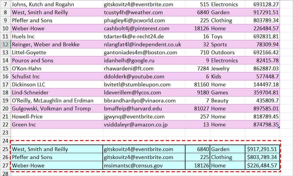
- Firstly, copy the information from File 2 and paste them into File 1.
- Now, Highlight the cells you’ve just pasted with a color. It helps you identify the new values.
- Select the entire Columns and choose Conditional Formatting in the Home Tab.
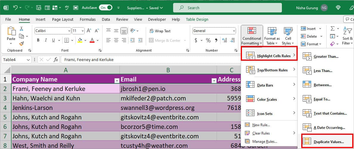
- Navigate to Highlight Cells Rules > Duplicate Values.
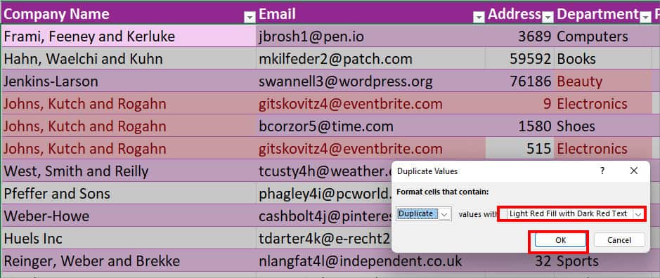
- On the Duplicate Values window, next to the value with, you can expand the drop-down and choose a Color. Click OK.
Step 2: Filter and Delete Duplicate Values
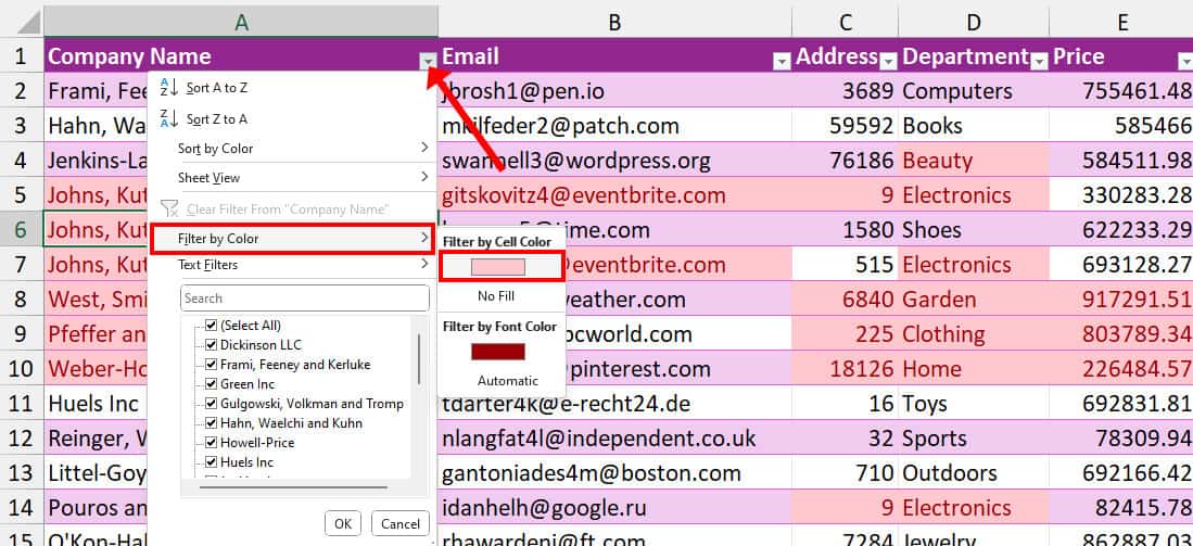
Now, you can use the Filter tool to filter out the values based on the color and delete them.
- Click on a cell within the data.
- If you don’t have a filter on, press Ctrl + Shift + L to enable it. Select Filter by colour > Filter by Cell Colour.
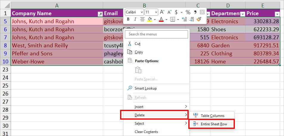
- Now, select the entire Filtered Data. Choose Delete > Entire Sheet Row.
- Again, enter Ctrl + Shift + L to turn off the Filter.
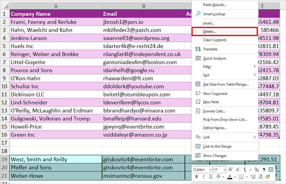
- Select the Pasted Data. Right-click on it and pick Delete.
Use Power Query Tool
Apart from importing various external files, the Power Query tool is also best to format your columns. You can sort, transform, split, group, and add columns in the Power Query Editor window. Here, you can find the Remove Duplicates option too.
Keep in mind, Power Query Tool is case-sensitive which means it takes “nisha,” “NISHA,” and “Nisha” differently. This means the tool would only delete duplicates if the range contains “nisha” and “nisha.’ So, if you want to mark such lowercase and uppercase values as unique, this method is for you.
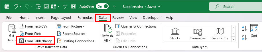
- On your worksheet, click Data Tab.
- Hover over the Get & Transform group and select From Table/Range.
- If Create Table window pops up, tick the box for My table has headers and hit OK.

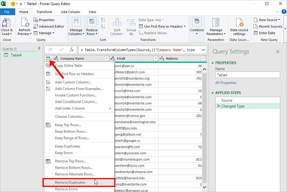
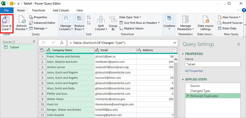
- On the Power Query Editor window, click on the Table icon > Remove Duplicates.
- Now, from Home Tab, choose Close & Load to import the table into a sheet.
Use UNIQUE Function
For users who do not want to delete duplicate values from the range itself, you can use the UNIQUE function. As the function name itself says, you can extract only the unique items with this function.
Also, since the UNIQUE function is not case-sensitive, it considers the lowercase and uppercase letters differently. For example, if your duplicate values are “Account,” “ACCOUNT,” and “account,” the UNIQUE function will extract the first item “Account.”
Syntax: UNIQUE(array, [by_col], [exactly_once])Example: Suppose, we need to draw out the unique items from cell A2:E22. To do that we entered the formula as below.
=UNIQUE(A2:E22)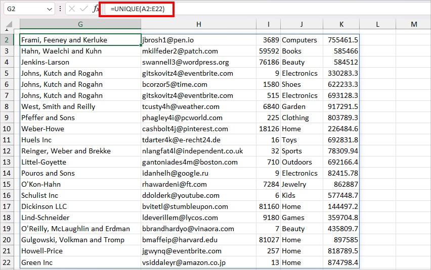
The Formula excluded all the duplicate values and returned only the unique ones.