While dealing with data in Excel, duplicate items can confuse you and lead to miscalculations. For example, you might end up concluding a total “of 12 Participants” in a competition when, in fact, there are “10 Participants.”
This is why knowing how to count only Unique and Distinct Items from the data is an important skill.
Also, even though the words “Unique” and “Distinct” may seem similar, there’s a major difference between them.
So, first, we will dig into what each value means such that you get a precise unique count for your data. Then, you can follow the methods as needed.
Distinct Vs Unique — Know the Difference
Although while counting unique items, your only motive is to exclude the duplicate values, you must know the difference between “Unique” and “Distinct” first.
Why? Because for each count, you’ll get a different result.
If you want to count only single items from the lists, it means “Unique.” For example, in the list (Outlook, Excel, Excel, Microsoft Word), Outlook and Microsoft Word are unique items. So, when you count, it’ll result in 2.
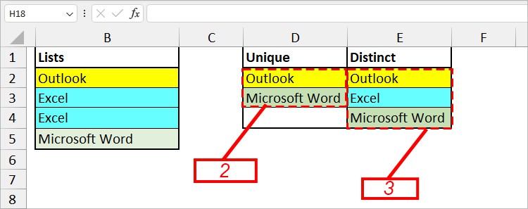
On the contrary, “Distinct” means counting the separate or different Values only. For Instance, again, in the same lists (Outlook, Excel, Excel, Microsoft Word), Outlook, Excel, and Microsoft Word is a Distinct item. So, the count result would be 3 this time.
How to Count Unique Values in Excel?
Count Unique Values in Column
Assuming you have a list of text strings in a single column, I will use the SUM, IF, and COUNTIF nested together to perform this.
| Functions Used | Syntax | Description |
| SUM | =SUM(number1, number2,…) | Returns the sum. |
| IF | =IF(logical_test, value_if_true, [value_if_false]) | Check logical test and return value when the condition is met or not met. |
| COUNTIF | =COUNTIF(range, criteria) | Count and return the total cells based on a criteria. |
Formula:

=SUM(IF(COUNTIF(range, criteria)=1, value_if_true, value_if_false))
Example:
Suppose, I have lists of names from cell B2 through B8. Let’s ignore duplicates and return only the unique items. For that, I used the below formula.
=SUM(IF(COUNTIF(B2:B8, B2:B8)=1, 1, 0))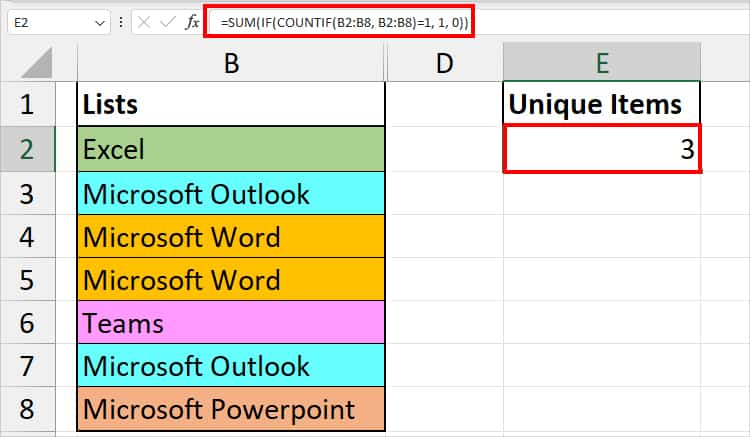
In the COUNTIF function, we have specified the formula to count only single items. The IF function returns 1 when the test is true and 0 when not. Finally, the SUM function returns the total count of numbers resulted by the IF function.
Since Excel, Teams, and Microsoft Powerpoint are unique, the formula returned 3.
Count Unique Text Strings or Numbers Only
There can be instances when you have both numbers and text strings in the Column.
Count Text Strings Only
To exclude numbers and count only text strings, we will use the SUM, IF, ISTEXT, and COUNTIF functions.
If you’ve noticed, here, only the ISTEXT function is extra. The rest of the functions are the same as above.
Formula:

=SUM(IF(ISTEXT(value) * COUNTIF(range, criteria)=1, value_if_true, value_if_false))
Example:
Here, I have lists of Columns including duplicates of text values and numbers. Let’s count only the unique names from the column.
=SUM(IF(ISTEXT(B2:B10)*COUNTIF(B2:B10,B2:B10)=1,1,0))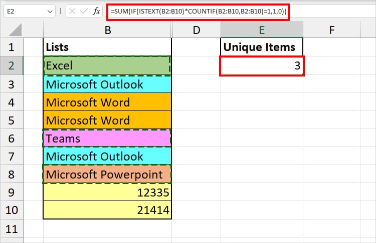
In the formula, by inserting the ISTEXT function, we have set the formula to take only texts. So, for output, we got 3.
Count Numbers Only
Similarly, now, let us count only the unique numbers from the lists. This time, I’ll enter the ISNUMBER function instead of ISTEXT.
For that, here’s the formula I will be using
=SUM(IF(ISNUMBER(B2:B10)*COUNTIF(B2:B10,B2:B10)=1,1,0))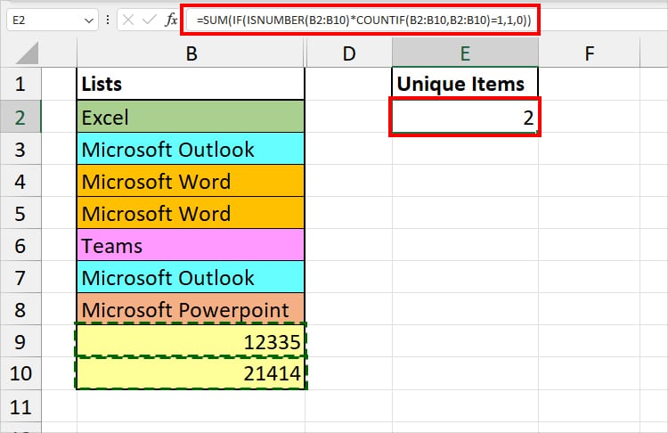
The formula counted unique numbers and resulted in 2.
Count Case-Sensitive Texts
In both above cases, the formula does not take the case-sensitive texts differently. So, if you want to count only the case-sensitive unique values, here’s the formula you can use.
=SUMPRODUCT(1/COUNTIF(B2:B8, B2:B8))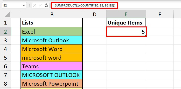
As a result, I got 5.
How to Count Distinct Values in Excel?
Since we already discussed what Distinct values mean above, let us now look into the formulas to count them.
Count Distinct Values in Column
To count the Distinct Values in the Column, we will use the COUNTA and UNIQUE functions nested together.
Example:
Here, I have lists of items with Duplicates. To count and return the distinct values, enter the formula below.
=COUNTA(UNIQUE(B2:B10))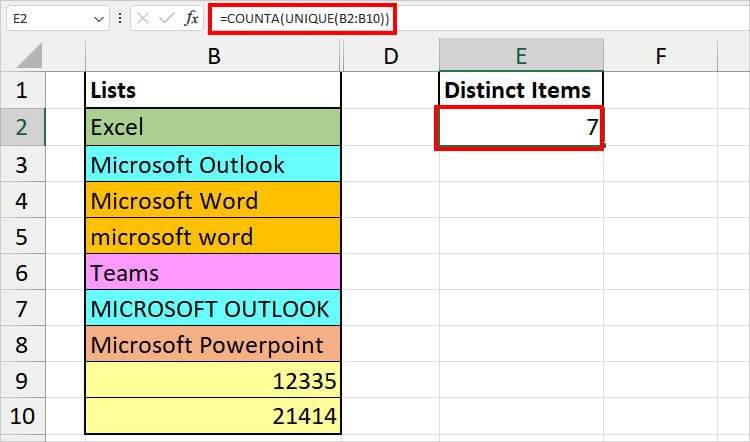
The formula counted all distinct texts and numerical items. Then, returned 7.
Count Distinct Texts or Numbers Only
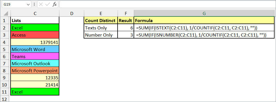
Let’s assume, you need to count only distinct numbers or texts only from the range.
| Count | Formula | Example (Formula) | Description |
| Distinct Texts Only | =SUM(IF(ISTEXT(range), 1/COUNTIF(range, range), “”)) | =SUM(IF(ISTEXT(C2:C11), 1/COUNTIF(C2:C11, C2:C11), “”)) | The formula excludes duplicates and counts all the distinct Texts within the C2:C11 range. It ignores the numerical values. We got 6. |
| Distinct Numbers Only | =SUM(IF(ISNUMBER(range), 1/COUNTIF(range, range), “”)) | =SUM(IF(ISNUMBER(C2:C11), 1/COUNTIF(C2:C11, C2:C11), “”)) | By using the ISNUMBER, we have specified the formula to only look for numbers and count distinct ones. The formula resulted in 3. |
Count Each Distinct Values
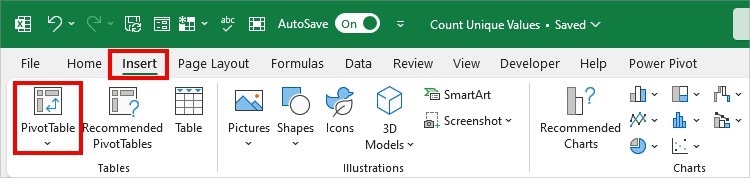
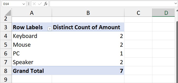
Assuming you need to identify each count of distinct values. To do that, you can use the Pivot Table.
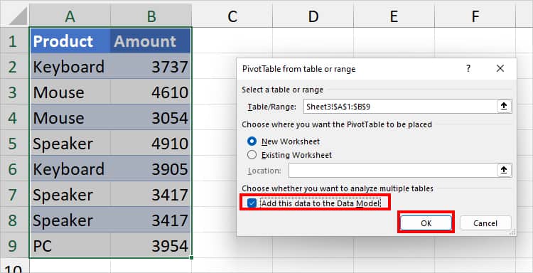
- On your sheet, select ranges.
- Click on Insert Tab > Pivot Table.
- Tick the box for Add this data to the Data Model and click OK.
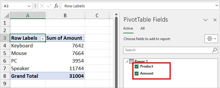
- Now, go to Another Sheet. On PivotTable Fields, checkmark Ranges.
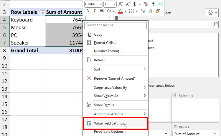
- Select all Sum of Amount Columns in PivotTable and right-click on it. Choose Value Field Settings.
- Below Summarize the value field by, pick Distinct Count and click OK.
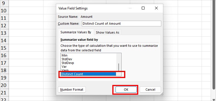
- You’ll see the Distinct Count of Amounts for each item.
Count Distinct Values Based on Criteria
Next, you can also count the Distinct Items based on a criteria. For example, count the number of unique items that are equal to VBA. It is similar to counting items based on 1 column.
To do that, we will nest the IFERROR, ROW, UNIQUE, and FILTER functions together.
Example:
From the given data, let’s count the names which is equal to VBA. Here’s the formula
=IFERROR(ROWS(UNIQUE(FILTER(D9:D15,E9:E15 =G6))), 0)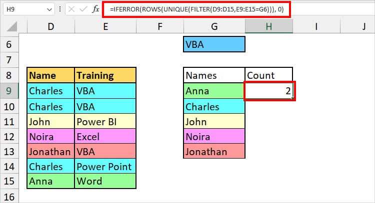
In this formula, we have specified the FILTER function to filter out the names with VBA. The UNIQUE function then discards the duplicates. Finally, the ROWS function returns the total row. In case the formula returns an error, we have set the IFERROR to return 0.
Here, we got 2.
Count Distinct Values Without Blank Cells
While counting, many formulas take blank cells as unique and include them too.
Therefore, for users having a blank cell, there’s a separate formula to exclude empty cells and count only the non-blank cells.
I know the formula may seem a bit long and intimidating. But, here, we are just using the SUM, IF, FREQUENCY, LEN, and MATCH functions nested together.
This is the formula I used to skip blank cells when counting the unique. Remember, it will count both Unique Texts and Numbers.
=SUM(IF(FREQUENCY(IF(LEN(D9:D15)>0, MATCH(D9:D15, D9:D15, 0), ""), IF(LEN(D9:D15) > 0, MATCH(D9:D15, D9:D15, 0), ""))>0, 1))We got 3 as a result.
Let’s take the formula simply as =SUM(number1, number 2) function and break it down to understand it.
Number 1: IF(FREQUENCY(IF(LEN(D9:D15)>0, MATCH(D9:D15, D9:D15, 0), “”)
- IF(LEN(D9:D15)>0, MATCH(D9:D15, D9:D15, 0): The IF function tests the LEN(D9:D15) > 0 condition. When the condition is met, it returns the position resulted the MATCH function. Or, “” null string when the value is False.
- IF(FREQUENCY(IF(LEN(D9:D15)>0, MATCH(D9:D15, D9:D15, 0), “”): Here, the FREQUENCY function returns the occurrence number of values. Then, again, IF function returns 1 when the FREQUENCY(IF(LEN(D9:D15)>0 condition is TRUE. It returns “” for FALSE value.
Number 2 : IF(LEN(D9:D15) > 0, MATCH(D9:D15, D9:D15, 0), “”))>0, 1)
In this formula, the IF function tests LEN(D9:D15) > 0 criteria and returns the position number resulting from the MATCH function when the condition is true. In case, the condition is false, it results in “” null string.
Finally, the SUM function adds the numbers and results in the total unique counts without the empty cells.
Count both Distinct and Unique Values with Power Query
If you want to count both Distinct and Unique items at once, use Excel’s Power Query feature.
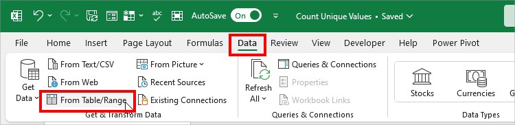
- Simply select your data and head to the Data Tab.
- From the Get & Transform Data group, click on Get Data. When prompted, choose Yes.
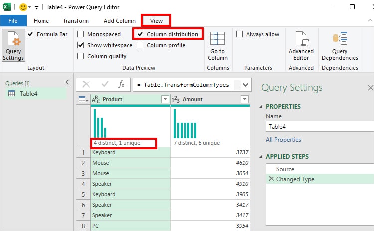
- Now, on the Power Query Editor window, navigate to the View Tab. Check the box for Column Distribution. It’ll show the total number of distinct and unique items.
By now, you must have learned how to count unique and distinct items. If you find the need to find the duplicates, we have a detailed article on “How to count duplicates in Excel.”