Conditional Formatting in Excel—Detailed Guide

As the name suggests, conditional formatting in Excel simply means applying certain formatting to cells based on some condition. 

However, unlike format painter, which also helps you copy and apply formatting to other cells, conditional formatting is dynamic. Meaning, it will automatically change the formatting of a cell even if its value changes in the future.

With several built-in conditional formatting options, you can highlight certain cells to make them stand out visually. At the same time, you could discover some interesting trends and patterns in a large dataset without breaking a sweat.

Using Built-in Options

Excel provides a list of several most basic and frequently used conditional formatting options under the Home tab. These options are easy to use and quite self-explanatory, which cover formatting dates, text, numbers, and so on. 

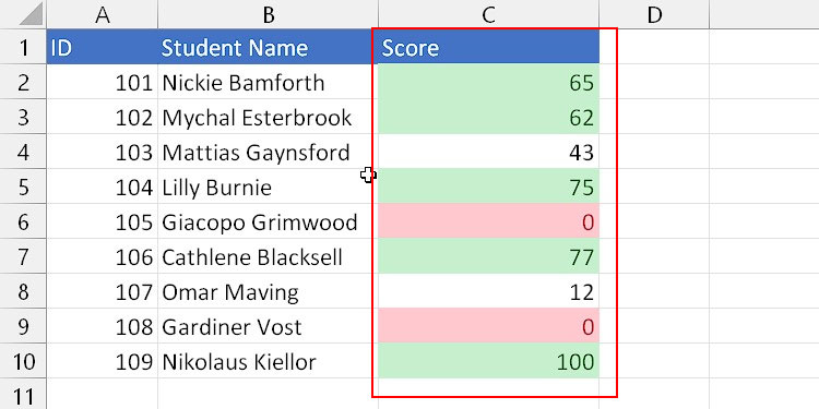
Highlight Cells Rules

These rules include common use cases like highlighting cells with values greater, less, or equal to another specified value. Also, you can highlight cells with a specific text and number, including duplicate values. 

In the image below, we will use the “Greater than” option to highlight cells having values greater than 60 with a green background.

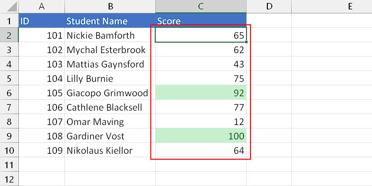
Top/Bottom Rules

By default, the rules in this section display the top/bottom 10 values (in numbers and percentages) among the selected cells. You can also specify a different number of items or percentages if you want.

Example: 
Here, we will be highlighting the top two scores with a green background.

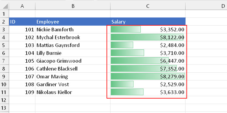
Data Bars

These options calculate the total percentage for each selected cell based on the highest value and display it in terms of data bars. Here, the longer data bar represents cells with higher values and vice-versa.

Example: 
In the image below, we will use data bars to visualize salaries ranging from low to high.

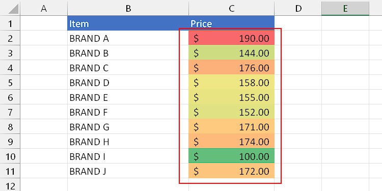
Color Scales

These rules display different colors or color gradients for each selected cell ranging from highest to lowest value. 

Example: 
Here, we will use the data bars to indicate the price of items ranging from cheap to most expensive with colors like green, yellow, orange, and red.

Icon Sets

These options display different icons based on how much percentage each selected cell value constitutes out of the total. The icon sets include icons like flags, arrows, circles, ratings, etc. 

Example: 
Here, we will use the up/down arrows to indicate positive or negative growth depending on whether the cell value is less or greater than 2%. Meanwhile, the right-facing arrow will indicate those having a growth rate equal to 2%.

Using Formula

Apart from the built-in conditional formatting options, you can use a custom formula to highlight cells that match your specific criteria (s). 

For instance, you can apply conditional formatting to an entire row based on the values in a particular column.

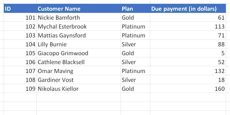
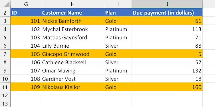
Here, we are trying to highlight the whole row containing customers that are subscribed to the “Gold” plan using conditional formatting.

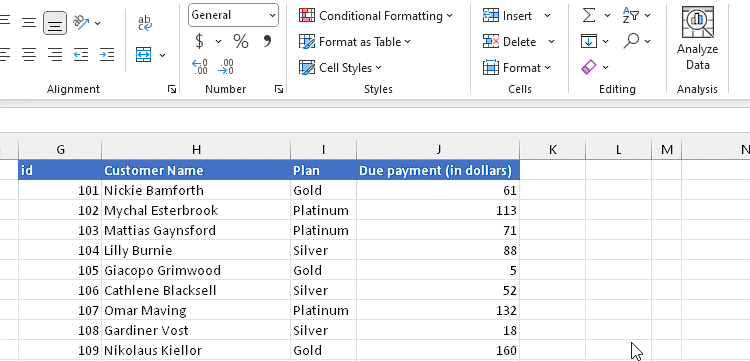
Now, we could use one of the built-in options, specifically the “Text that Contains” option.  However, such a rule formats only the cells with the “Gold” value instead of highlighting an entire row. It doesn’t work even if we select all the customer data. 

So, we need to enter a custom formula in this particular case.

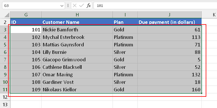
1. Select all cells containing the dataset values. 
   
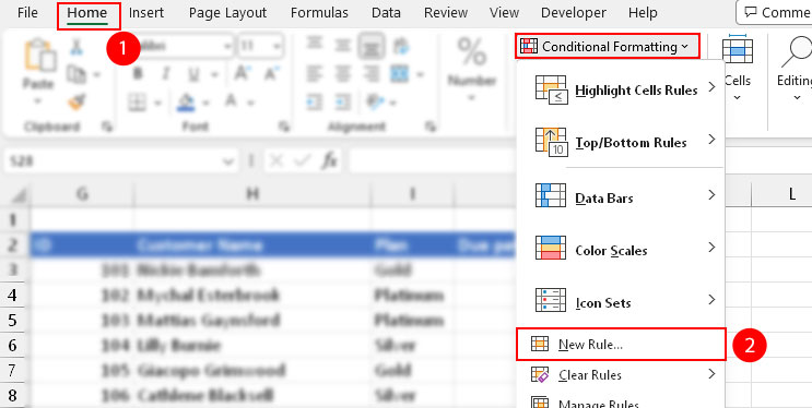
2. To apply conditional formatting with a formula, click Conditional Formatting and select New Rule.
   
3. Then, select the Use a formula to determine which cells to format option.
4. Type =$I3=”Gold”. Here, the first entry under the Plan column is I3. So, we used mixed cell referencing ($I3) to lock the “I” column and consider only the cells under the Plan column. Similarly, we used relative referencing starting from row 3 to apply formatting to the entire row.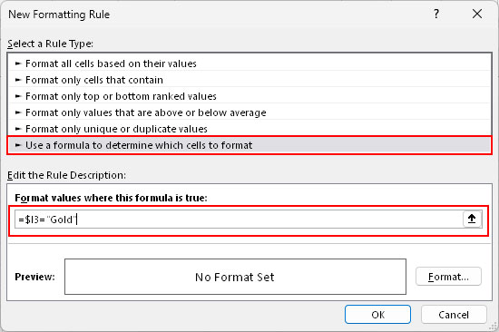
   
5. Now, click Format and choose an appropriate fill or font color.
   
6. Click OK.

The final result is as follows.

Using a similar approach, you can format every first, second, or nth row according to your specific condition. On top of it, you can even format duplicate rows using conditional formatting.

How to Apply Conditional Formatting Based on Multiple Criteria?

In case you need to apply conditional formatting based on multiple conditions, you can do so using logical operators like AND and OR.

For instance, in the previous example, we applied formatting to an entire row based on one condition — whether the cell contains the “Gold” value or not. 

However this time, we’ll apply formatting to the entire row only depending on multiple conditions.

Using AND function

Using the logical AND function, you can apply conditional formatting to cells only if they match all the conditions.

For instance, format an entire row for customers that have the Gold plan with a due payment of more than 60 dollars.

Here, the formula is
=AND($I3="GOLD",$J3>60)=

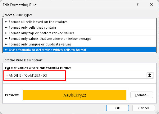
After using the AND function inside the formula, the result is as follows:

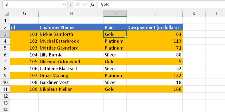
Using OR Function

Using it, you can apply conditional formatting to cells only if any one of the conditions returns TRUE.

For instance, format an entire row for customers that have either a Gold or platinum plan.

Here, the formula is
=OR($I3="GOLD",$I3="Platinum")

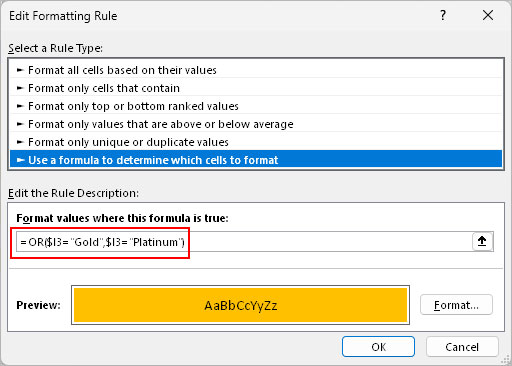
After using the OR function inside the formula, the result is as follows.

Bonus Tips

• If you convert your cell range into a table, Excel will automatically extend and apply the conditional formatting rule to new entries inside the table.
• Along with regular cells, you can even use conditional formatting for pivot tables and charts.
• While using the “Highlight Cells Rules” and “Top/Bottom Rules” options, you can also enter a cell reference instead of manually inputting the value.

Related Questions

How to Find and Remove Conditional Formatting?

If you later decide to remove conditional formatting from your worksheet, you can find all of them inside the Conditional Formatting Rules Manager. Then, you can delete or even choose to edit the rule from there. Just select Conditional Formatting > Manage Rules under the Home tab.