Excel’s XLOOKUP function beats all the other lookup functions in terms of features and functionality. It is by far the best alternative to VLOOKUP, HLOOKUP, INDEX and MATCH functions.
I know when you look into such big formula at first, you may get intimidated not knowing where to start. But, I’ll guide you through the examples of how to use this function from a very beginner to an advanced level. You can also find tips and tricks to avoid errors.
Benefits of Using XLOOKUP Functions
- The return value is not just limited to one item. XLOOKUP can return a number of arrays from the lookup table.
- The function can look for values on both the right and left of the lookup value. So, the lookup value can be in any row or column.
- You can use XLOOKUP to search values in both vertical and horizontal arrays.
- XLOOKUP can perform a binary, reverse, or default start search.
- When the value is not found, you can enter a “Message” to return to instead of the #N/A error. So you wouldn’t have to use the ISERROR or IFERROR for this.
- XLOOKUP supports multiple criteria.
Tips to Use the XLOOKUP Function
- To conduct Binary Search Modes, your texts must be sorted in A to Z and Z to A order. For the numbers, they should be either in ascending or descending order. Else, you’ll get an error.
- I recommend you enter the if_not_found in every XLOOKUP formula to avoid receiving errors.
- If you need to type a Text in the formula argument, enclose them within the “” (Double Quotation).
- XLOOKUP function is not at all case-sensitive.
- Avoid having unwanted spaces and characters in the Lookup value.
- You can use Named Ranges or Named Table in the formula to shorten the formula length.
Arguments Used in the XLOOKUP Function
Excel’s XLOOKUP function has a lot of arguments compared to the other lookup functions. However, all the arguments are not compulsory. Some of them are optional too.
Syntax: XLOOKUP(lookup_value, lookup_array, return_array, [if_not_found], [match_mode], [search_mode])- lookup_value: Item you want to search
- lookup_array: Array that contains the Lookup value.
- return_array: Array to return from the lookup_array
- [if_not_found]: Text to return when the lookup item is missing.
- [match_mode]: Specify how you want to return the lookup value.
- 0: Exact Match or #N/A when no value found.
- -1: Exact Match or closest smaller value when value not found.
- 1: Exact Match or next larger value when value not found.
- 2: Wildcard Match.
- [search_mode]: Determine the search mode.
- 1: Start Search from the first value.
- -1: Reverse Search. Start looking for value from the last value.
- 2: Binary Search in ascending order.
- -2: Binary Search in descending order.
Applications of XLOOKUP Function
Example 1: Vertical and Horizontal Lookup
Firstly, we will just take a look into a simple example that illustrates XLOOKUP can return values Vertically as well as Horizontally. Here, we won’t go into depth with all the function arguments as I’ve discussed them one by one in other examples. I’ll just use the lookup value, lookup array, and return array to demonstrate this.
Example: Vertical Lookup
Let’s find out the Total Sales of Tim. For this, we used the formula as
=XLOOKUP(H2, A2:A5, E2:E5)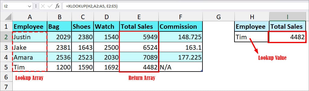
In the XLOOKUP, our Lookup value is H2, the lookup array is A2:A5, and the return array is E2:E5. Since our return array is a column, the formula looked for items vertically and resulted in 4482.
Example: Horizontal Lookup
Here, we have a table in the horizontal format. From the data, we will check the Task Status of the employee name “Steven.”
=XLOOKUP(A7, B1:G1, B4:G4)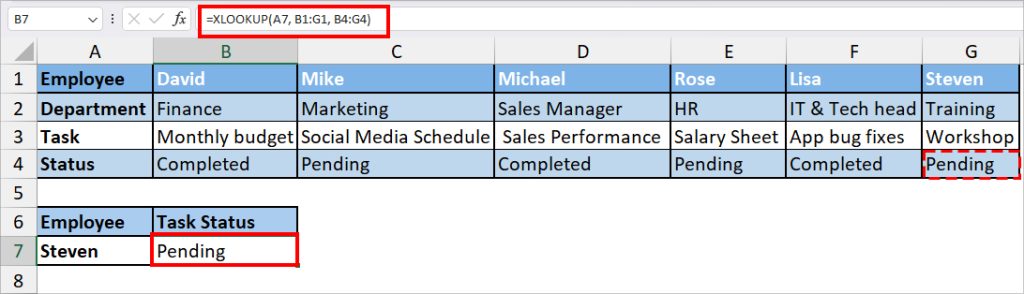
The above formula looked for Steven horizontally in the B1:G1 array and returned Task Status “Pending” from B4:G4.
Example 2: Exact Match
Using the XLOOKUP function, you can return the exact match from the lookup table. For this, we will pass down the 0-match mode in the formula.
In case, there are no values to return, you’ll receive a #N/A error. However, if you specify a message in the “if_not_found,” the formula will return that message instead of the error.
Example: Suppose, I have a table of Household Expenses. Let’s say I want to find out the Grocery amount for the month of May.
For this, I will enter the XLOOKUP formula as below.
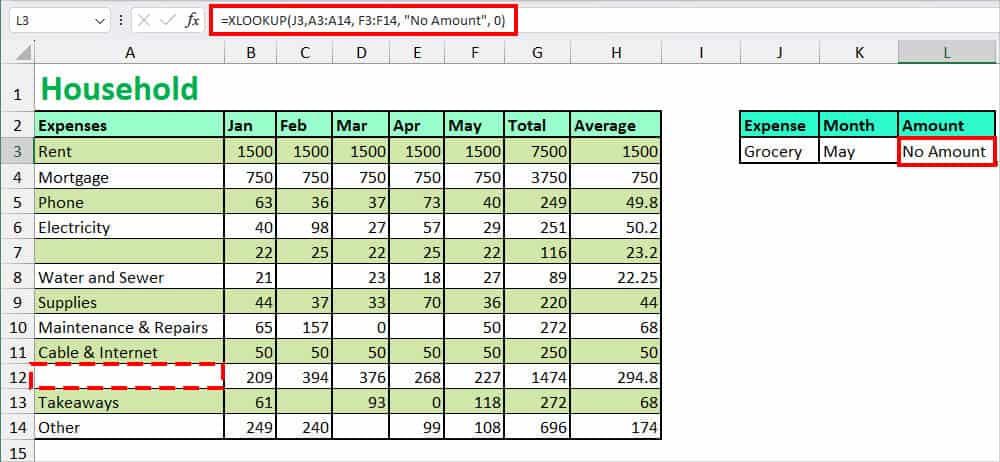
=XLOOKUP(J3,A3:A14, F3:F14, "No Amount", 0)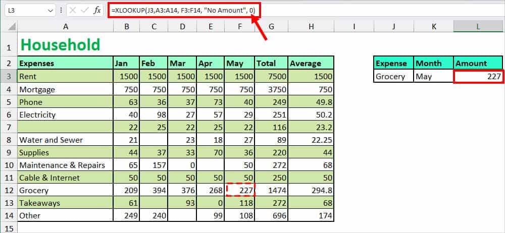
In the formula, our lookup_value is Grocery which lies in the lookup_array A3:A14. Similarly, our return_array is F3:F14. If there’s no exact match, we have specified the formula to return “No Amount.” Since we passed down 0 as match mode, the formula will return the exact item from the return array. As a result, the formula returned 227.
In case, there was no value, it would’ve returned “No Amount.”
Example 3: Approximate Match
For some data in Excel, an approximate match is more helpful than the error or if not found message. To return the approximate match, you can use either -1 or 1 match mode in the XLOOKUP function. We’ll discuss both of them in the example below.
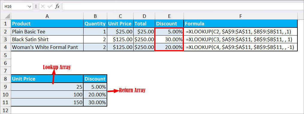
Example: Let’s say I want to return the discount percentage for the products based on their Unit Price. As there’s no exact value for Unit Price, I need to return the approximate match.
| Example | Formula | Output | Description |
| Exact Match | =XLOOKUP(C2, $A$9:$A$11, $B$9:$B$11, ,1) | 5% | Since there’s an exact match in the lookup value, it returned 5%. It implies even though you enter a partial match, the formula prioritizes and returns an exact item. |
| Approximate Large Number (1) | =XLOOKUP(C3, $A$9:$A$11, $B$9:$B$11, , 1) | 30% | In this case, the lookup value does not match the item in the lookup array. Here, we have specified the formula to return the closest large number. As a result, XLOOKUP returned 30% for the 125 unit price. |
| Approximate Small Number (-1) | =XLOOKUP(C4, $A$9:$A$11, $B$9:$B$11, , -1) | 20% | Again, we have the same lookup value as in example 2. But, this time, we passed down -1 match mode in the formula. So, the XLOOKUP formula returned the nearest smallest percentage which is 20%. |
Example 4: Partial Match
In the XLOOKUP function, you can use the Wildcard Characters to return the lookup values in a partial match. Remember, the Match_Mode 2 in the function argument? It returns the Wild card match.
There are three different Wild Characters and each of them represents their own meaning. If you’re a beginner, Wildcard can seem very complex at first. So, before you dive into the examples, I suggest you go through what each Wildcard Characters implies first.
P.S. In the given examples, we haven’t specified the search mode in the formula. So, the XLOOKUP formula will use the default Start search mode and return the first occurrence from the lists. We will discuss the different search Modes in more detail later with examples.
| Wildcard Character | Formula | Output | Description |
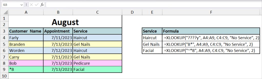
| ? | =XLOOKUP(“????y”, A4:A9, C4:C9, “No Service”, 2) | Haircut | In the XLOOKUP formula, we specified the “????y” as the look-up value. Now, if you see at the table there are two names that have the same number of letters and end with “y”. Since XLOOKUP looked from first, here, we got result for Farly. But, if you enter “C???y” as the lookup value, it would’ve returned Gel Nails. |
| * | =XLOOKUP(“B*”, A4:A9, C4:C9, “No Service”, 2) | Gel Nails | Since, our Lookup value is “B*”, it’ll return the Service for a customer whose name begins with B. In case, you passed down “*B” as the lookup value, it would have returned the service for the customer with the last letter as B. For example, “Pedicure” for Bob. |
| ~ | =XLOOKUP(“~*B”, A4:A9, C4:C9, “No Service”, 2) | Facial | In the formula, we’ve used the Tile in the lookup value to stop *B from functioning as Wildcard Character. As a result, it returned the service for *B value which is “Facial.” |
Example 5: Different Search Modes
If you’ve used VLOOKUP or HLOOKUP before, you must have noticed these functions returns the first occurrence in duplicate data by default. But, this is not the case in XLOOKUP. You can actually specify the search mode to look for values from last, first, ascending, or descending order.
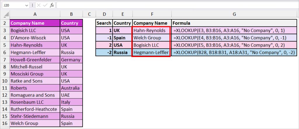
Example: Here, we have a list of Companies with duplicate countries. Let’s return the Company name for each Country.
| Search Mode | Formula | Output | Description |
| 1 (Start Search) | =XLOOKUP(D3, B3:B20, A3:A20, “No Company”, 0, 1) | Hahn-Reynolds | In the formula, 1 search mode will return the first instance from the duplicate value. So, for the UK country, we got Hahn-Reynolds. |
| -1 (Reverse Search) | =XLOOKUP(E4, B3:B16, A3:A16, “No Company”, 0, -1) | Welch Group | This time, we’ve entered -1 Search Mode in the XLOOKUP. The formula returned the last item which is “Welch Group” for Spain. |
| 2 (Ascending Order) | =XLOOKUP(E5, B3:B16, A3:A16, “No Company”, 2) | Bogisich LLC | If your Data is sorted in the ascending or A to Z order, use the 2 Search Mode. Again, just like the Start search, it also returns the first occurrence of the smallest number or first letter item. |
| -2 (Descending Order) | =XLOOKUP(B28, B18:B31, A18:A31, “No Company”, 0, -2) | Hegmann-Leffler | Here, we sorted the data in Z to A order first. Since we passed down -2 in the search mode, it returned the final value of Russia. It is similar to the Reverse Search but the data must be in descending or Z to A order. |
Example 6: Return Array
One of the specialties of the XLOOKUP function is that it can return multiple items from the lookup table. So, in this example, we’ll explore how to use the XLOOKUP to return an array.
Example: Let’s say, I have a record of Employee, Title, and Sales amount. Based on the Total Sales, I want to find out the Employee and Title.
To do so, I used the XLOOKUP formula as below.
=XLOOKUP(C3, C2:C8, A2:B8, "No Value", 0, 1)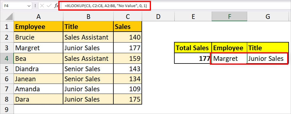
In the formula, I have passed down the argument to return the A2:B8 array(Employee and Title) for the C3 lookup value. So, I got Margret and Junior Sales as an outcome. If there was no exact match, it would have returned “No Value.”
Example 7: XLOOKUP Across Sheets
You can also use the XLOOKUP to extract an item from a different sheet. So, you don’t have to worry about transferring information to another sheet just to use the Lookup table. The best part is it creates a dynamic sheet reference between the worksheets.
Formula: = XLOOKUP(lookup_value, SheetName!lookup_array, SheetName!return_array, [if_not_found], [match_mode], [search_mode])Example: In a New sheet, let’s say I want to prepare a summary of Expenses. For this, I want to extract the information from each sheet before adding them. I entered the following formula.
=XLOOKUP(B3, Education!B2:F2, Education!B7:F7, "No Value", 0)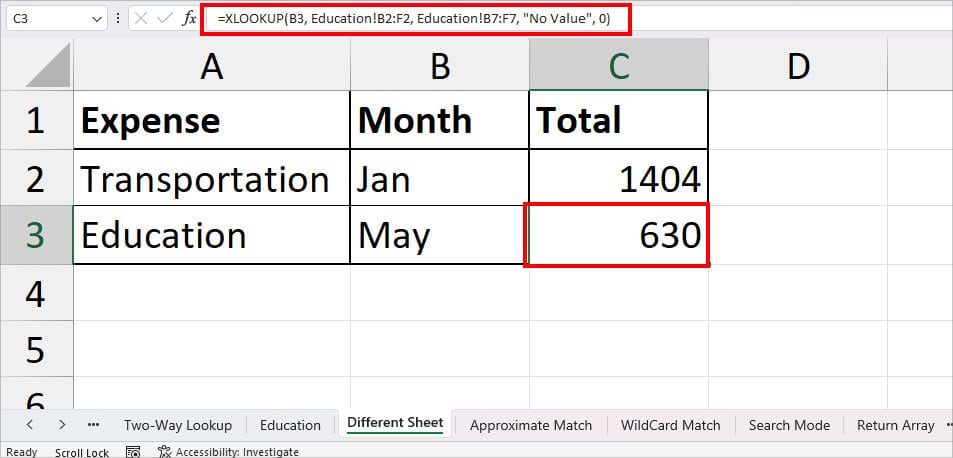
Here, the formula resulted in 630 for May.
While you can enter the formula manually, it’s a lot easier if you head to the source sheet and select the lookup and return array by yourself. Follow these tips to use the formula.
- In a new cell, enter =XLOOKUP(. Click on the lookup value cell and add a Comma.
- Head to the Source Sheet, and select the lookup array. Again, type a Comma.
- Now, select the Return array and enter a comma.
- Type in the if not found, match mode, and search mode arguments separated by a comma. Once you’re done, Close the bracket and press Enter.
Example 8: XLOOKUP with Different Workbooks
We’ve discussed the ways to use XLOOKUP with various conditions and criteria in the sheet from the above examples. But, there can be instances when you have information in the different workbooks and need to draw out data from there, right? To use the XLOOKUP to your utmost advantage, let’s use this function in separate workbooks.
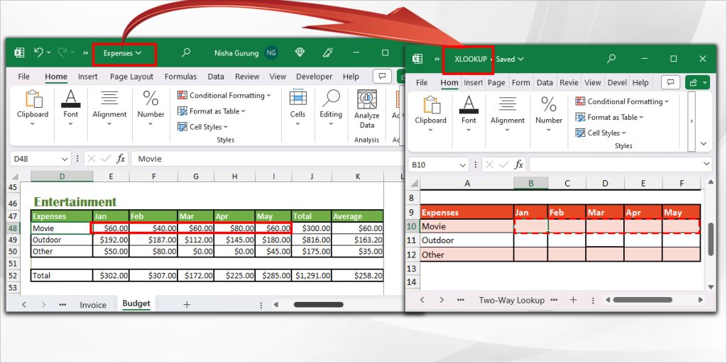
Formula: = XLOOKUP(lookup_value, [Workbook.xlsx]SheetName!lookup_array, [Workbook.xlsx]SheetName!return_array, [if_not_found], [match_mode], [search_mode])With all the formula arguments, sheets, and workbook names, the XLOOKUP function looks even more lengthy and complex. But, I’ll show you the easiest way to enter them. Before you start, open both source and destination workbooks.
Example: Let’s take, for instance, I have data about Entertainment expenses in the “Budget” Sheet of the “Expense” workbook. I need to draw out the cost of Movie expenses for all 5 months in the “XLOOKUP” workbook.
I used the given formula to achieve this.
=XLOOKUP(A10, [Expenses.xlsx]Budget!$D$48:$D$50, [Expenses.xlsx]Budget!$E$48:$I$50, , 0)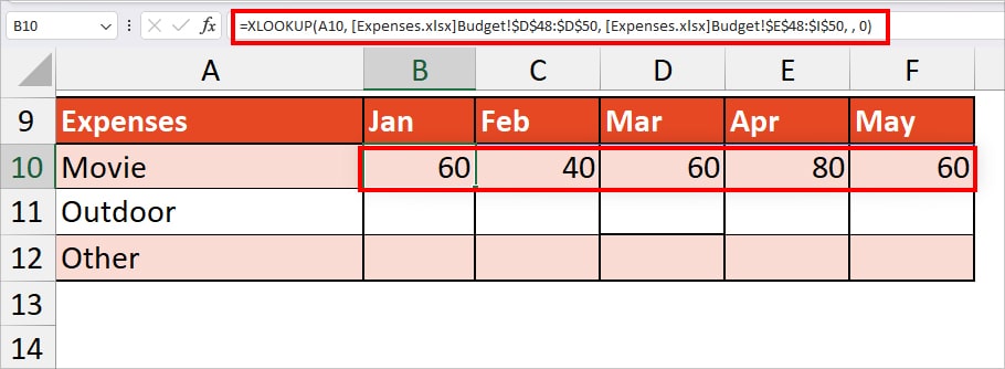
The formula returned an entire amount for the month of Jan, Feb, Mar, Apr, and May for Movie.
Here’s how I entered the formula.
- On the Destination workbook, enter =XLOOKUP(. Select a cell with a lookup value and type a comma.
- Now, go to another Workbook and click on the Sheet. Select the range with the lookup value.
- Enter a comma and select the cell ranges for the return array.
- Type in all the arguments separated by a comma. Close the bracket and hit Enter.
Example 9: Two-Way Lookup
So far, we learned a single lookup in all examples. Now, let’s learn the two-way lookup. For this, we will be nesting the XLOOKUP inside the XLOOKUP function. It is best when you need to return a value from the intersection of a Row or Column.
Formula: XLOOKUP(lookup_value1, lookup_array1, XLOOKUP(lookup_value2, lookup_array2, data_values))Example: Here, I have Education Expenses Data for different months. Suppose, I want to return the Amount of Miscellaneous for the month of February.
=XLOOKUP(I2, A3:A5, XLOOKUP(I3, B2:F2, B3:F5))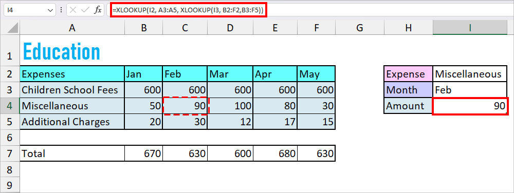
- XLOOKUP(I3, B2:F2, B3:F5): Firstly, this formula returns the Row of return array which is 600, 90, 30.
- XLOOKUP(I2, A3:A5, XLOOKUP(I3, B2:F2, B3:F5)): Then, the formula returns an item that matches the lookup value. As a result, we received 90.
Make XLOOKUP Function More Dynamic
While using the XLOOKUP function, do you change the lookup value in the formula every time? If you are, stop spending all of your time editing the arguments and let the formula recalculate itself.
There’s an efficient way to make your Function more dynamic. We will create a drop-down list for our lookup value.
- Select the cell that is your lookup_value.
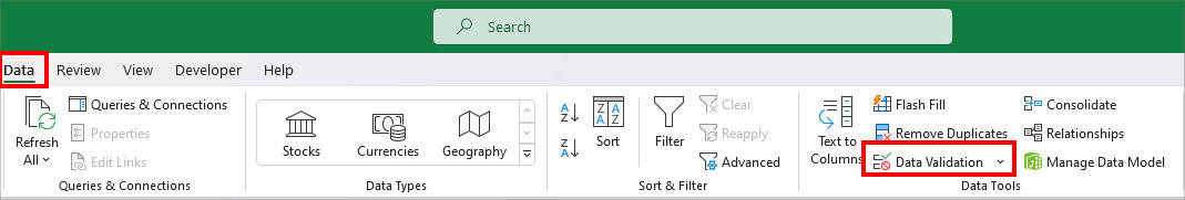
- From the Data Tab, click on Data Validation.
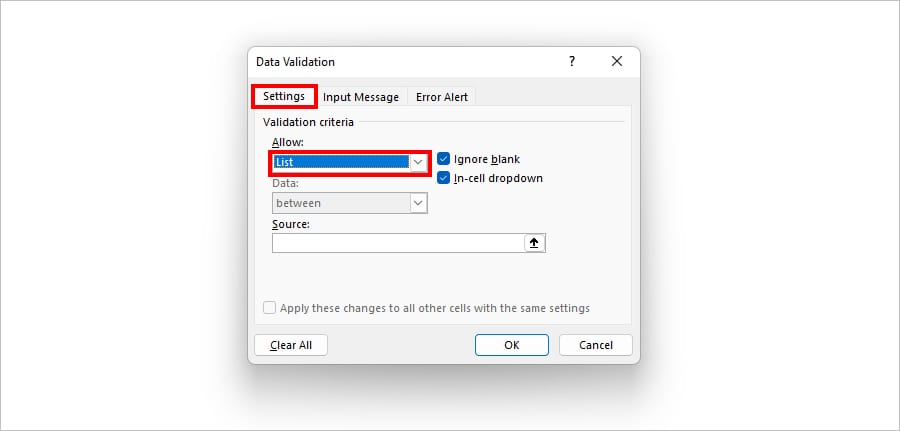
- On Data Validation dialogue box, be on the Settings tab. For Allow, click the drop-down list and pick List.
- On Source, click the Collapse icon and select the Lookup array. Click OK.
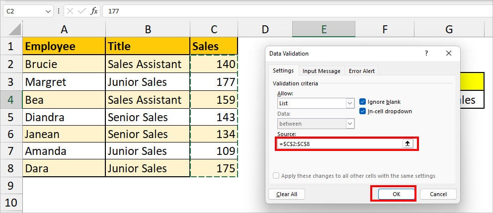
- Now, if I pick another Sales Value, it’ll return a different employee and title automatically.
Avoid Errors when using the XLOOKUP Function
When you use the XLOOKUP function, these are the common errors you may get. In most cases, it occurs when the arguments of the formula haven’t been referenced properly. But, if you know the cause, it isn’t a big deal to dodge those errors.
| Error | Probable Causes |
| #N/A Error | No Lookup Value. No Exact Match. Data not sorted as required while using the Binary Search. |
| #REF! | Deleted Column that was Return Array. Source Workbook closed when using the formula for separate workbooks. |
| #VALUE! | When the lookup array is vertical and the return array is horizontal or vice versa. |
| #NAME? | Text arguments without the “” |