How to Create and Use a Printable Form in Excel

While Excel has a Data Entry Form to record information for the owner, it certainly lacks the in-built printable forms that other users can fill. For example, the Feedback Form, Employment Survey Form, Student’s Review Form, and so on.

However, you can easily make the fillable and printable Forms on your own with just the Data Validation tool, Check Boxes, and VLOOKUP formulas. 

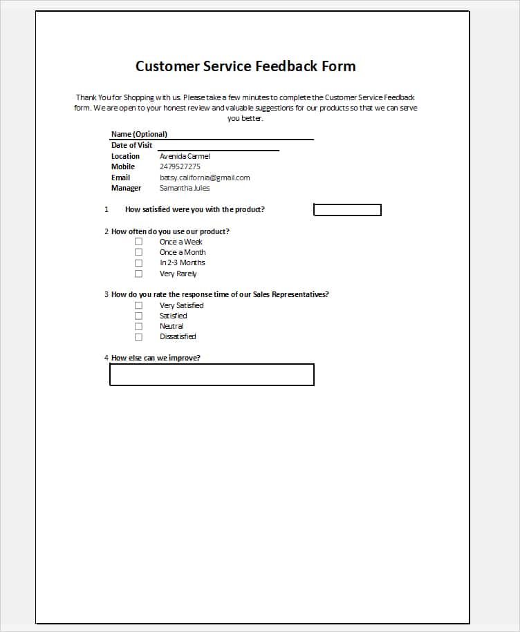
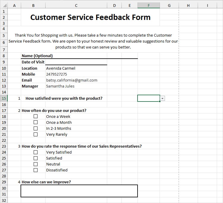
Here, as an example, I will be creating the Customer Service Feedback Form from scratch.

Step 1: Prepare a Form Outline

• Set Page Size: Set a paper size in Excel to print the form. In the Page Layout Tab, click on Size > A4.
  You’ll see a grid line separating the page in Excel. Ensure to work within that area only.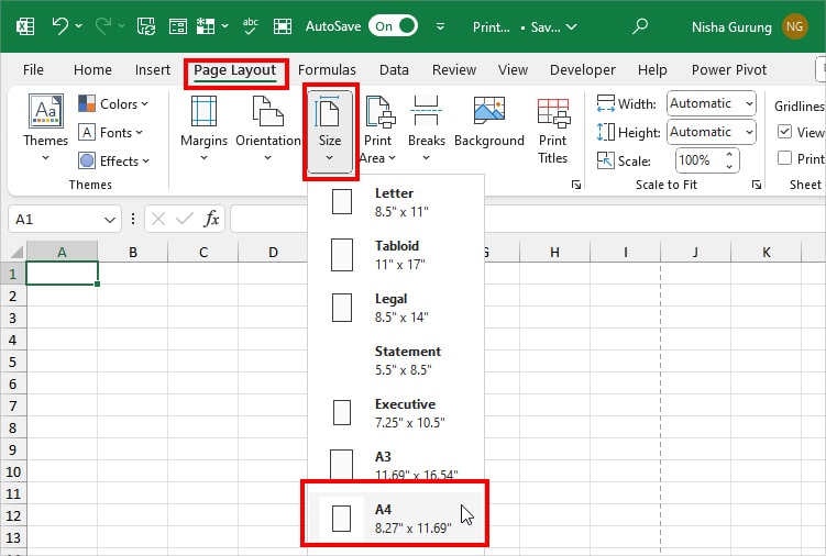
  
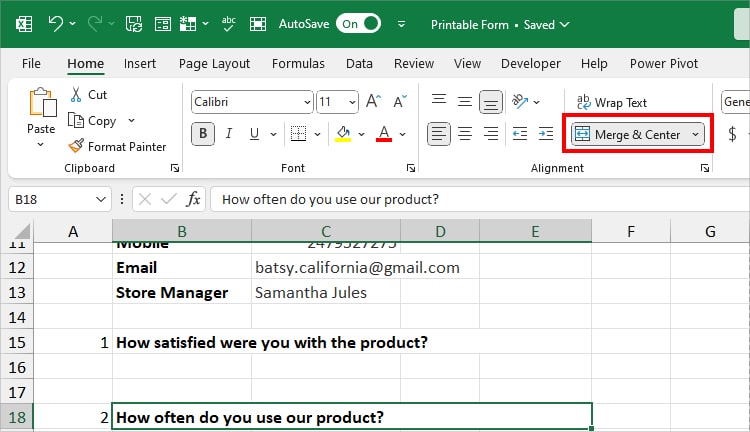
• Heading: Use Merge & Center for a certain range to make a space for the Heading. Type the Form Title.
  Then, adjust the Color, Font, Alignment, and Font size from the Home Tab. After that, you can also add Pictures or Logo in the Heading.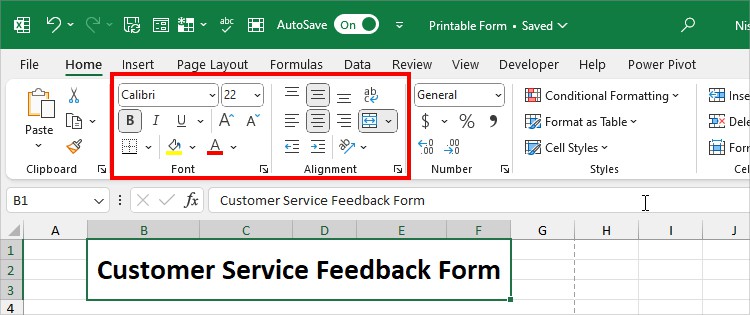
  
• Participant’s General Information: This step is optional and solely depends on your Form Type.
  I have entered the Name and Date of Visit. Again, for this information, you can format texts and font styling as you wish.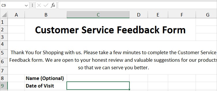
  
• Apply Bottom Border: Since the cell gridlines will be gone while Printing your form, apply the Border where required.
  Here, I will use the Bottom Border for the general information we just entered above. Select Cell Ranges. Expand Border menu > Thick Bottom Border.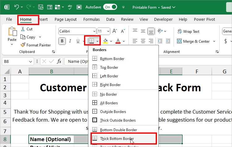
  

Step 2: Create a Form

According to Form type, there can be many elements you can incorporate in the Form. For Instance, a Check box, a Drop-down list, Option Button. Or, you can leave the field for participants to manually type the answer. 

I’ll add all of these elements in my form below. 

Use Drop-down list

1. Merge cells and type in the Question. 
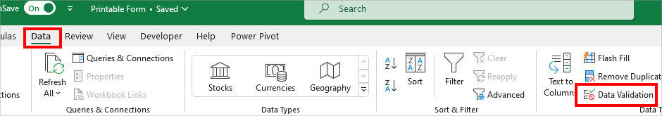
2. Next to Question, select a Cell. From the Data Tab, click on Data Validation.
   
3. In the Data Validation window, expand the drop-down menu for Allow and choose List. On Source, click the Collapse icon and select the data source. Here, mine is on =Sheet2!$C$4:$C$7. Hit OK.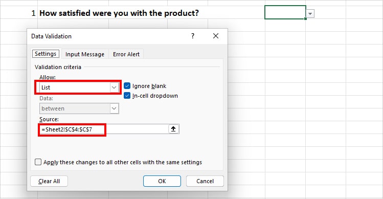
   
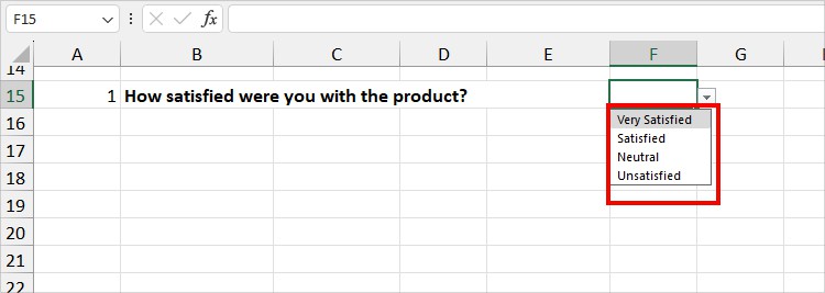
4. Now the Participant has an option to pick Very Satisfied, Satisfied, Neutral, and Unsatisfied.
   

Use Drop-Down List and Formula

Next, you can also use a drop-down list and a VLOOKUP formula to auto-populate the options in Excel Spreadsheet.

For Example, when a customer chooses Location, other information like the Mobile, Email, and Store Manager gets filled automatically. You can do the same for any information as required.

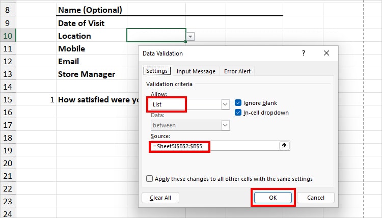
1. Next to the information, select a Cell. From the Data tab, click on the Data Validation.
   
2. Below Allow, choose List. On Source, click the Collapse icon and select the Data references in another sheet. Then, Hit OK.
   
3. Now, enter the formula =IFERROR(VLOOKUP(C10, Table1, 2, 0), ""). Here, we have specified the VLOOKUP to return the exact item for lookup value (drop-down list cell) from the second column. To replace the formula error, we have specified IFERROR to return the null string.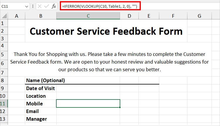 
   
4. Again, use the same IFERROR and VLOOKUP formula for the rest of the cells. Make sure to change the column index in the formula.
   
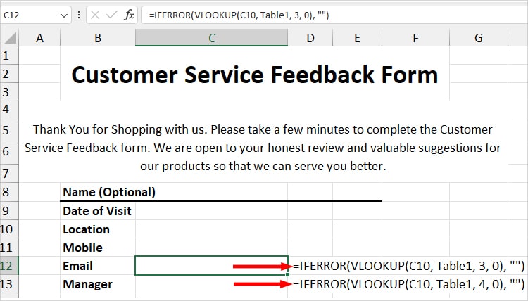
5. Now, when you choose a value in the drop-down list, it’ll fill in all the remaining information.
   

Use Check Box/Option Button

For the Next question, I will add multiple options and a check box next to it. You can also choose to insert the Option Button. The steps are the same.

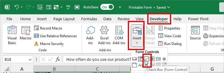
Before starting, you will need to load the Developer Tab first. 

1. Select Cell Ranges and Merge them. Type a Question.
   
2. Choose a Cell and head to the Developer Tab. Click Insert and pick the Check Box or Option Button below the Form Control.
   
3. Draw the Check Box. Then, remove the text and keep only the box.
   
4. Copy the Check Box and Paste them as required. Line up the Boxes in each Cell to dedicate to each Option.
   
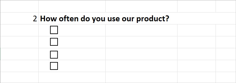
5. Next to the Checkboxes, I’ll now enter my Options List.
   

Now, complete the rest of the Form using the Drop-down lists or the Check Boxes.

Step 3: Format Form and Print

• Hide the Sheet with the information that you used for Reference. See our Hide or Unhide Excel Sheets for an Advanced guide. 
• Put Away Gridlines from the Sheet. For that, navigate to the View Tab. In the Show group, untick the Gridlines option and hit OK. 
• You can lock cells in the Spreadsheet where you wouldn’t want the users to make changes.
• Once the Form is ready, save the workbook. Then, enter Ctrl + P keyboard shortcut to print that form. We have covered all the things you should note while printing a worksheet in the “How to print a Worksheet on Excel Sheet” guide.