How to Filter Based on a List in Excel

Usually, we filter data based on a single item in Excel. But, did you know that you can filter your sheet based on entire lists at once?

Yes, there are various Excel tools and functions to achieve that. For example, you could filter a table based on several car records. Or, filter lists with multiple criteria such as a column of cars and colors. 

Also, in this article, I will walk you through the steps to make your filter process more dynamic for a smooth and productive work performance. 

Using AutoFilter

If you have shorter lists to filter your data, you could use the AutoFilter tool itself. It’s the easiest way to filter without using any complex formula. 

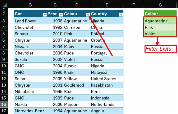
Suppose, let us consider that I have only 3 values in the lists to filter my data.    

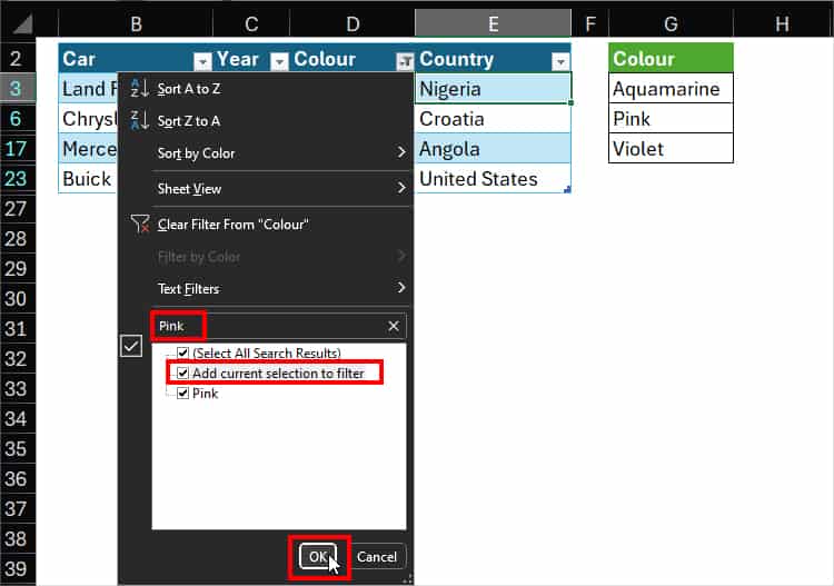
1. Click on the Filter button in the Column.
   
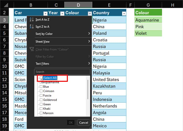
2. On the AutoFilter Lists, tick on Select All to deselect all items.
   
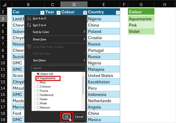
3. Now, check the box for the first item and click OK. Here, I ticked on the Aquamarine.
   
4. Again, expand the Filter. Type the next item. Then, checkmark for Add current selection to filter. Click OK.
   
5. Repeat step 4 for all the items in the lists. If you want to organize your data, click Filter and choose Sort Order.
   

After you’re done, you can remove the Auto Filters.

Use Advanced Filter

As mentioned, for large lists, you would have to type and tick boxes repetitively with the above approach. So, for users who have multiple values in Column to filter your data, I recommend you use Advanced Filter.

Here, you can define both the Filter range and the Criteria Range. Moreover, you will also have the option to import the filtered data in different locations. 

1. Select your Data table.
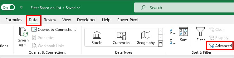
2. On Data, click Advanced.
   
3. On the Advanced Filter window, choose your Action option which is to Filter the list, in-place or Copy to another location.
   
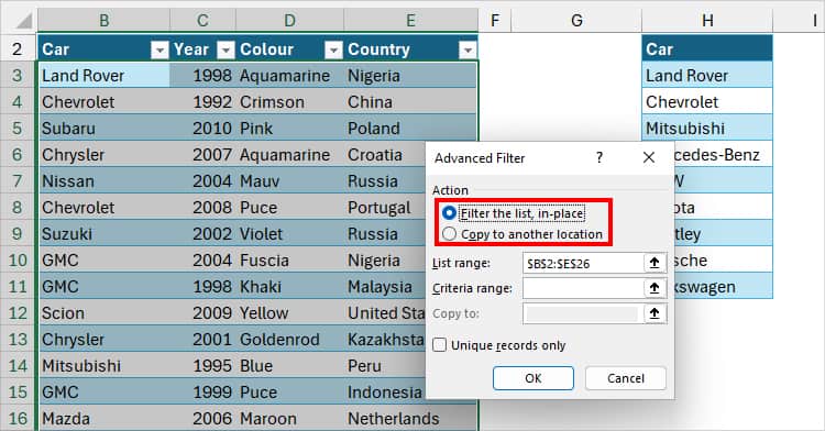
4. On the Criteria range, click the Collapse icon and select your Column Lists.
   
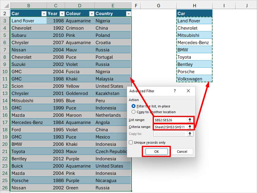
5. Click OK. You will have the filtered items on your Sheet.

Using COUNTIF Formula

If you’re comfortable using the formula, the COUNTIF function is even more dynamic. Here, we will insert a new column as a helper and use it as a base to filter items. This method is also best if you have lists in another sheet.

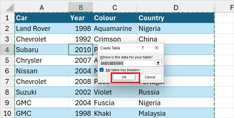
Syntax: =COUNTIF(range, criteria)

Firstly, apply a Table Format for your source and criteria data. Click on a cell and press the Ctrl + T shortcut on your keyboard. On the prompt, pick OK. 

Tables are dynamic and automatically include newly added rows. It’s even better if you name a table as it makes sheet referencing simpler in the formula. 

Now, next to your last Column, enter this formula. 

=COUNTIF(ct[Car], [@Car])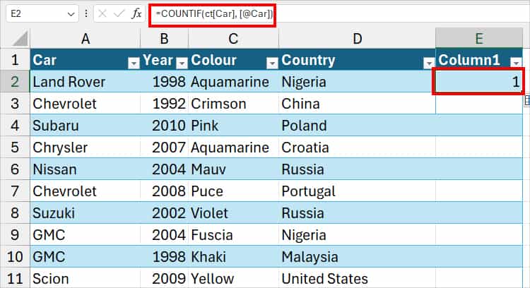

In the formula, ct[Car] is a criteria table range in Sheet3. Similar [@Car] is the first cell of the source table. I have specified the COUNTIF to count the texts of ct[Car] range that matches with [@Car] table.

The formula will result in 1 or 0 if there’s a unique list in your criteria table. After you get the output, drag down the Auto-Fill curosr to apply the formula to all. 

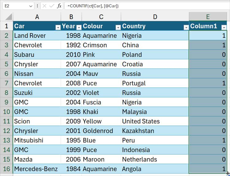
Now, to filter your data based on criteria lists, click the Filter button in the COUNTIF column. Untick the box for 0 and click OK.

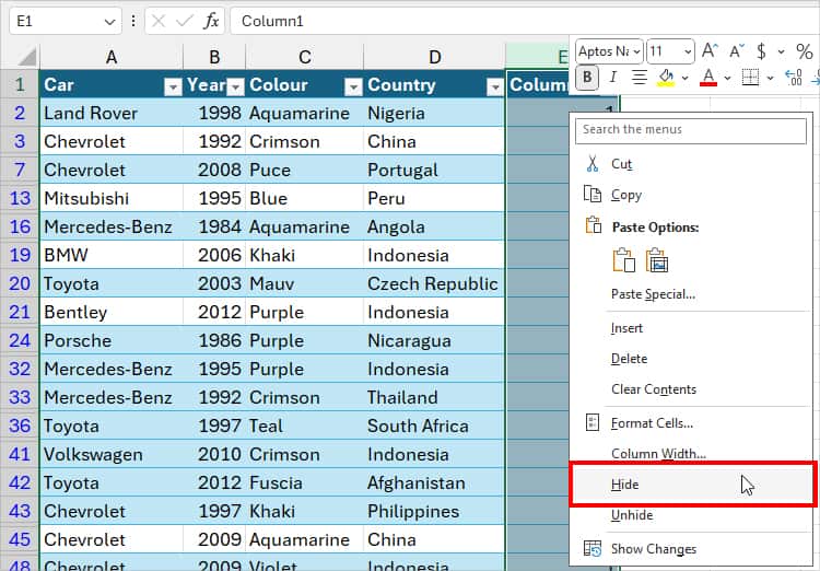
If you don’t want the helper column in your sheet, you could hide it. Select the Column Header. Right-click on Column and choose Hide.  

Use Drop-Down Lists and FILTER Function

Next, another way to filter data based on lists is to make a drop-down list and use the FILTER function.

Now, this method is slightly different from the approaches we’ve discussed above because you can choose to display only one criterion at a time from the lists.

We will also delve deeper into the filtering items with two or more lists. 

Insert Drop-down list

1. Click on empty cell.
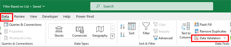
2. On the Data tab, choose Data Validation.
   
3. On the Settings tab, choose the List option for Allow. 
   
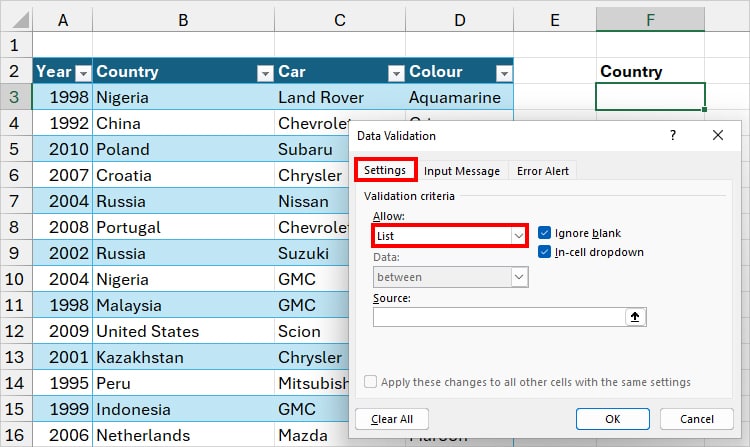
4. In the Source field, select the Criteria Column with the Collapse icon and hit OK.
   
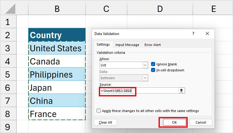
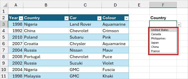
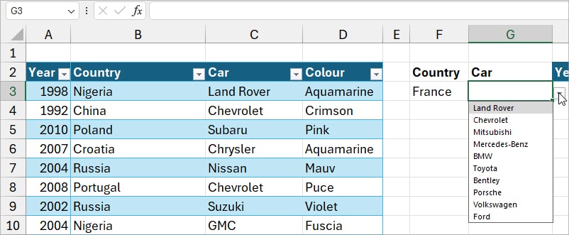
5. Here’s the Drop-down list.
   

Use FILTER Function

To filter data based on lists, we will use Excel’s FILTER Function now. You could use it for a single or multiple criteria. 

Syntax: =FILTER(array, include, [if_empty])

Single Criteria 

Now, enter this formula to return the filtered ranges. Make sure there are empty ranges for output. Else, you’ll encounter #SPILL! Error.

=FILTER(Table8, Table8[Country] =F3, "No Data")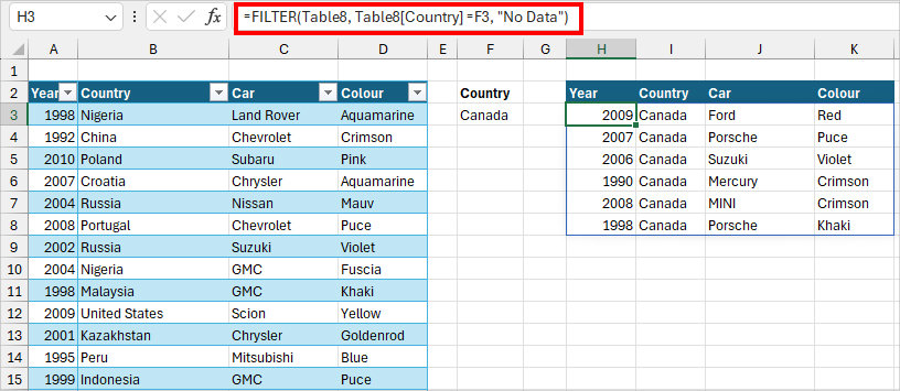

Here, in the filter function, I have passed down the argument to return the items from the table range when the Country Column matches the value in F3. In case there isn’t a match, the formula would return “No Data” Output.

Just like that, you can expand the drop-down and pick another value to show the data for that country only.  

Multiple Criteria

To narrow down your data filter, you can include the Multiple Criteria in the FILTER function.

For Instance, I filtered my data based on the country lists above. But, I can also choose to filter out the country and car at the same time. 

Let’s assume I already have my drop-down lists ready for Car. Use Data Validation to create for your records.

Now, this time here’s the formula.

=FILTER(Table8,(Table8[Country]=F3)*(Table8[Car]=G3),"No Data")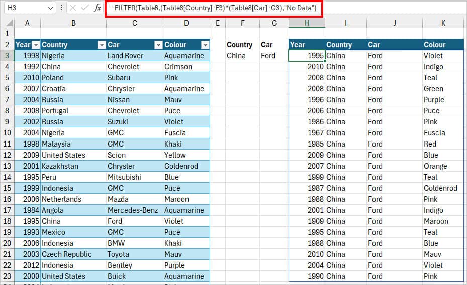

In the formula, (Table8[Country]=F3) is criteria 1 and (Table8[Car]=G3) is criteria 2. The filter function returns an array from Table8 for the given condition. 

But, in case there’s no value, the formula would return “No Data.” Choose the Value in the drop-down lists as needed.