How to Do a Horizontal Filter in Excel

While there is Excel’s Filter tool to filter out the values in a specific condition, the feature is limited to columns only. Meaning, you cannot filter items based on rows.

But, we do have several workarounds that’ll help you to filter the horizontal data.

Using FILTER Function

If your data is arranged horizontally, you should use excel’s Filter function. This function has extended functionality that even supports multiple criteria to filter within a range.

Syntax: FILTER(array, include, [if_empty])

The FILTER function takes up mainly three arguments. 

• array: Data Ranges to filter 
• include: Boolean array. The height and width of the array should match with the array.
• [if_empty]: Returned value when the array is empty. 

The argument with [] parentheses are optional.

Example: Suppose I have a row of Employee, Department, Task, and Status. Let’s filter the horizontal data in different criteria.

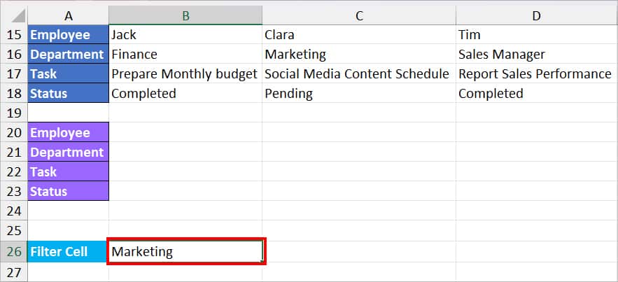
First, we will create a helper cell and dedicate that cell to set criteria. As the FILTER function is dynamic, the value you change in the cell will automatically update the filter accordingly. So, we’ve assigned a cell B26 and entered “Marketing” to filter it.

Now, to filter the marketing, we used the formula as

=FILTER(B15:M18, B16:M16 = B26, "No Value")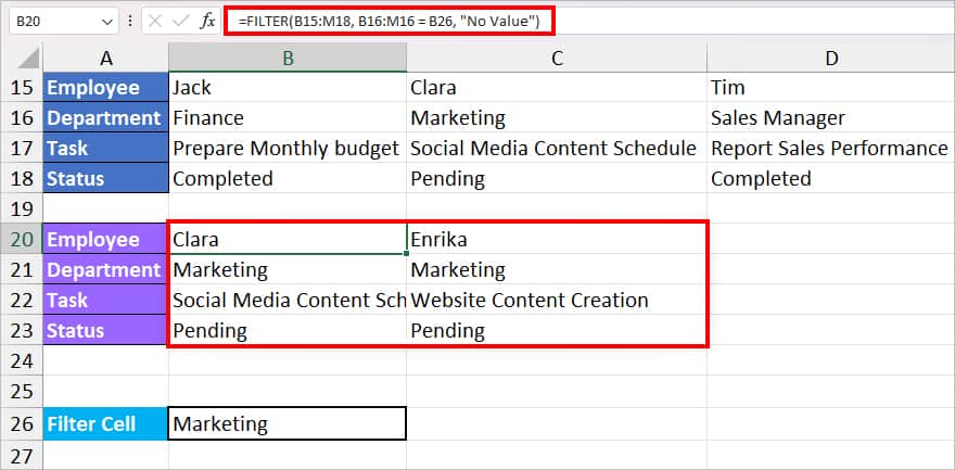

In the above formula, we have passed down the cells B15 through M18 as our array to filter data. We have specified the criteria to filter out the Marketing department. In case the array is empty, the formula will return “No Value.” Since there are values, the formula returned all the items of the Marketing Department.

Now, if you enter Finance in the filter cell B26, you’ll get the filtered value of the Finance Department. 

Use the FILTER and TRANSPOSE Function

In case you do not have data in horizontal order, you can use the FILTER and TRANSPOSE functions nested together to filter values. The TRANSPOSE function returns the values switched from rows to columns and vice versa. So, you could apply a filter without changing the data arrangement.

Example: Let’s say, you want to filter out the value of the Marketing Department horizontally. For this, you can enter the formula as

=TRANSPOSE(FILTER(A2:D11,B2:B11="Marketing","No Value"))

It’ll return all the values of the Marketing department. Let’s break down the formula to understand how it worked.

• FILTER(A2:D11, B2:B11=”Marketing”, “No Value”): In this formula, we have specified the FILTER function to filter values of the Marketing department which lies in cell B2:11. The function will look for all the items with the Marketing department and return employee name, department, tasks, status in columns just like in the original data. In case there is no value, it would return No Value.
• TRANSPOSE(FILTER(A2:D11, B2:B11=”Marketing”, “No Value”)): Now, the TRANSPOSE function switches the rows and columns of the returned value.

Transpose Data and Use Filter Tool

Since the FILTER function might not be available in older Excel versions, you could manually transpose data. Then, use the Filter tool as you would usually. 

Excel’s transpose tool will change all existing rows to columns and vice versa. So, after you transpose the data, the filter will apply to the horizontal data. Here, you do not have to use any formula. So, this method is also for users who do not want to use the FILTER function. 

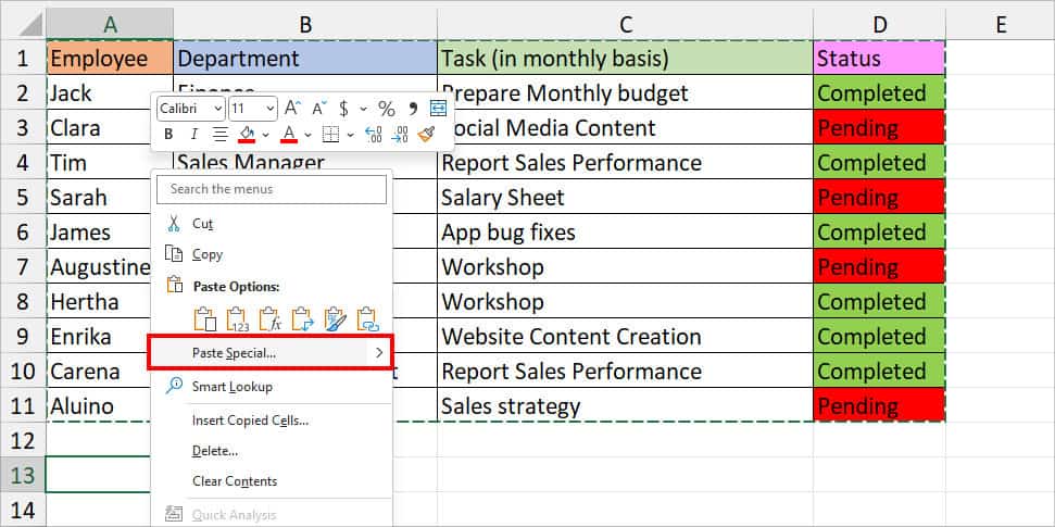
1. On your worksheet, select your data and enter Ctrl + C key to copy the data.
2. Right-click on a new cell and choose Paste Special.
   
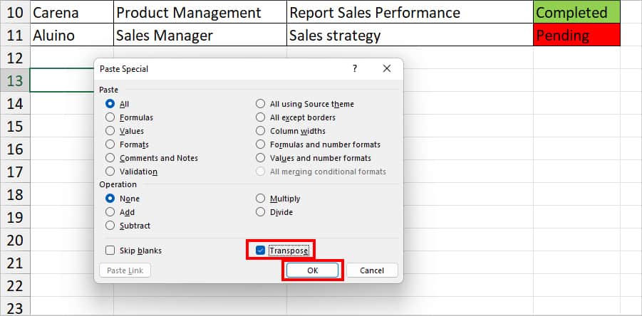
3. On the Paste Special window, tick the box for Transpose and click OK.
   
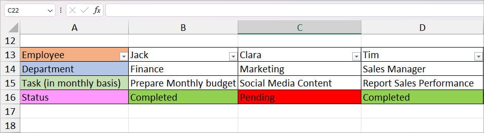
4. You’ll have the transposed data in your sheet. Click on the Cell and enter Ctrl + Shift + L shortcut key to turn on Filter.
   
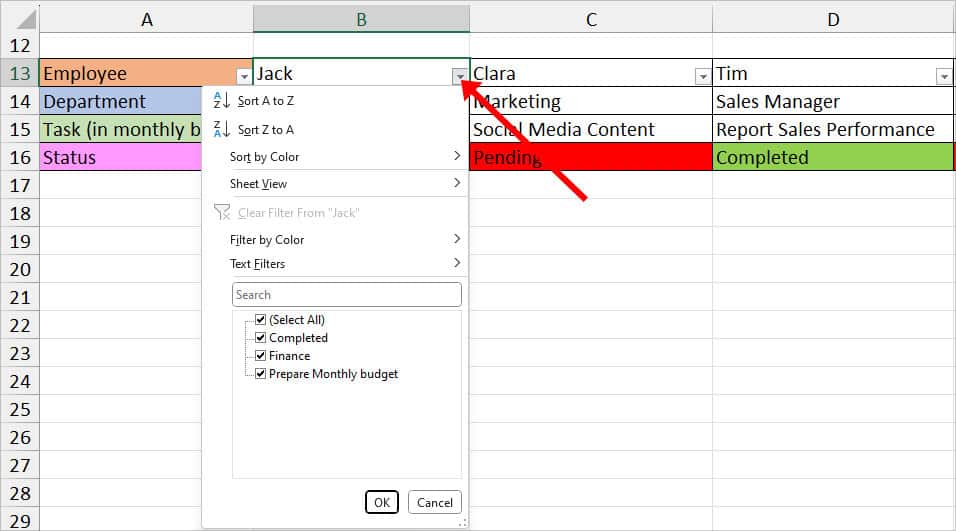
5. Click the Filter icon in any one column. Then, filter data as required.
   

Create Custom Views 

Another way to filter horizontal data is by using a custom view. Here, we will hide columns and create multiple custom views of data arranged horizontally. Then, in the end, we will selectively choose to show only one custom view to filter data. 

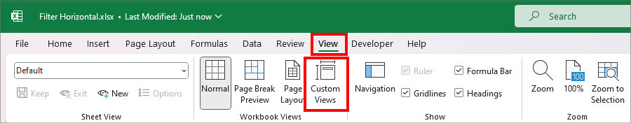
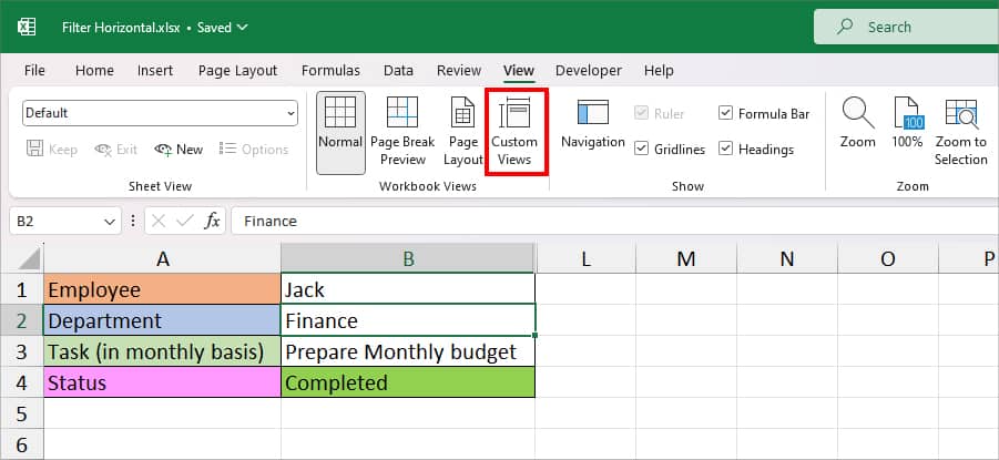
1. On your Excel sheet, click View Tab.
2. From Workbook Views Section, click on Custom Views.
   
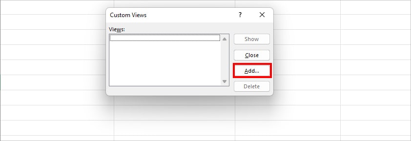
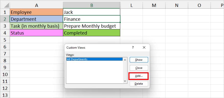
3. On the Custom Views window, click on Add.
   
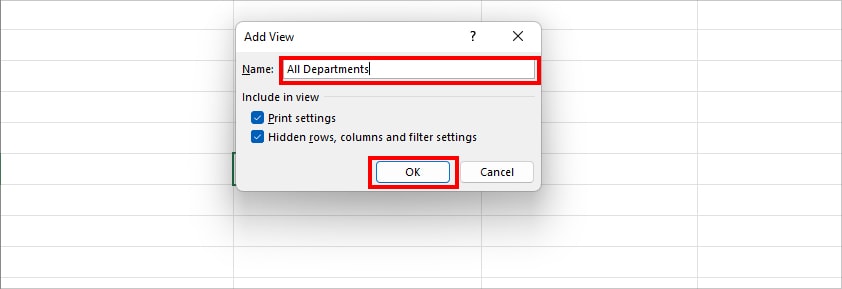
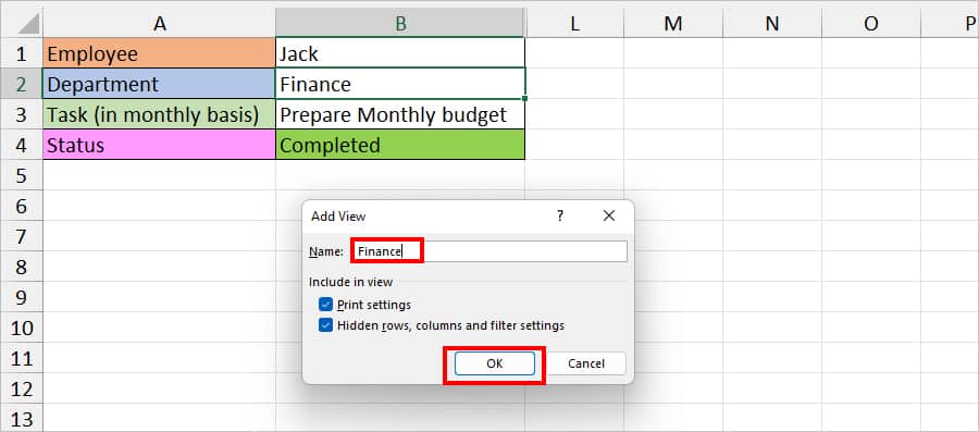
4. On Add View Window, enter the Name and hit OK.
   
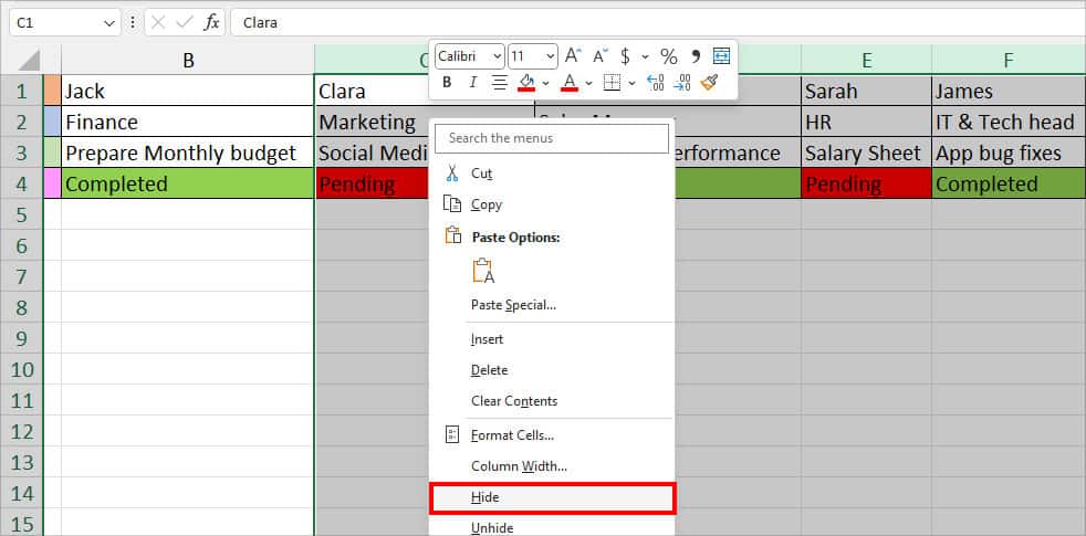
5. Again, to create a custom view for a specific department, hold down the Ctrl key and select all other columns. Leave the column you want to filter. As an example, we will add a Custom View of Finance.
6. Right-click on the Selected column and choose Hide.
   
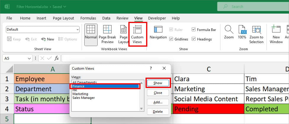
7. Now, from the Workbook Views, click on Custom Views.
   
8. On Custom Views, click Add.
   
9. Type in a new name in the Add View and hit OK.
   
10. Repeat Steps 5 to 9 to add up a new Custom View for other departments.
    

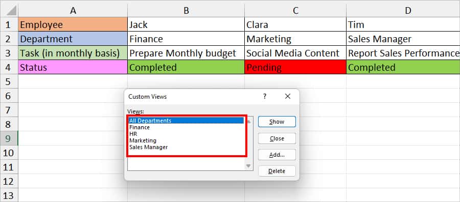
Now, you can choose to show only one of the custom views at a time. Suppose, you wish to filter the Finance department. For this, click on Custom Views in the View Tab. On Custom Views, select Finance and choose Show.