How to Name a Table in Excel

By default, Excel names each table sequentially with the initial name set as Table1. And, as you create more tables, they will be named Table2, Table3, and so on. However, such names don’t give out any information about what type of data the table contains and are not helpful to the user. To avoid this problem, you can name your tables. 

Doing so doesn’t only give an idea about the table contents but makes them more accessible as you can reference a specific column or the whole table data while writing formulas.

In addition to the table name, you can also apply several table design formatting to make the data even more informative.

Some Essential Naming Conventions while Naming a Table

Before you begin naming your tables, there are certain rules such names must follow.

• The name must start with alphabets.
• The name cannot contain any space characters. You can instead use underscores. For example, table_Customer, table_Address.
• The name cannot start with special characters like +,-, &,*, etc.
• The name must be unique. This means Excel interprets Customer and customer as the same name.
• The name cannot be a cell reference like B8, or B$8.

From the Table Properties

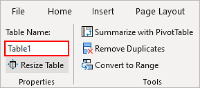
After you convert a cell range into a table, a separate “Table Design” tab appears at the top menu. You can use it to quickly name the table.

1. Select any cell on the table.
2. Click the Table Design tab.
   
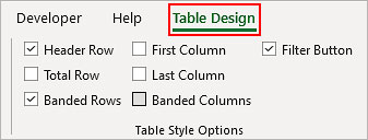
3. On the top left corner, replace the default table name (Table1, Table2, or similar) with the preferred name and press Enter.
   

Using the Name Manager

The Table Design tab only shows the name of the selected table. So, for some reason, you don’t have an idea of where the required table is, you can use the Name Manager as all the tables in the whole worksheet appear there.

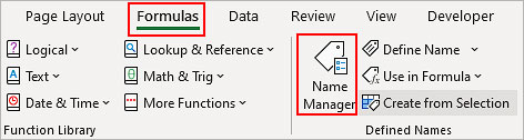
1. Go to the Formulas tab.
2. Click Name Manager. You can find it inside the Defined Names section.
   
3. On the next window prompt, click New.
4. Enter a preferred name for the table next to the Name field.
5. Additionally, select the scope and enter your comment.
6. Click the Up arrow icon and select your table.
7. Click OK.

How to Update a Table Name?

If you ever need to update the table name later, you can do so using the Name Manager. However, you can only edit the name and comments. Other properties like the cell reference and scope of the table are greyed out and unavailable.

So, you have to move the table into the desired location first and then name it.

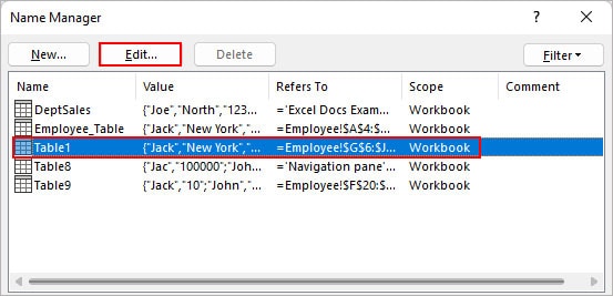
1. Click Name Manager under the Formulas tab.
   
2. Click the Filter button and select Table Names.
   
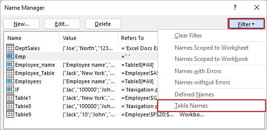
3. On the next window, select the table name you want to update and click the Edit button.
   
4. On the Edit Name window, replace the previous name with the new name.
   
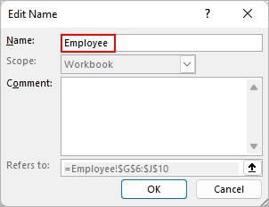
5. Click OK.

Note: Using the name box, you can find the list of all the named ranges and tables. However, unlike a named range, you cannot name a table with it. Also, after you convert a named range into a table, it still has a table name. So, you can reference the cell range by both the named range and table name.

How to Use a Table Name in a Formula?

Once you have a table name, you can reference it in a formula and use it as a dynamic named range. Meaning, the table automatically includes any new entries on the table without needing to change the table cell reference.

Also, you can access a column inside the table. For that,  you simply type the square bracket and Excel automatically displays the list of existing columns in that table.

For instance,

The above table is named “Employee_table” and we want to calculate the total salary of all the employees. So, we use the SUM function here.

Now that we have the table name, we can use it inside the formula as follows.

=SUM(Employee_Table[Salary])