How to Update or Edit an Entire Column in Excel? 8 Easy Ways

When working in Excel, you will often find the need to revise the formula or values in columns.

Normally, if there are a few cell ranges in the data column, you could edit cells one by one. But, on huge columns whose number spans more than hundreds and thousands, it’d be a wearisome process!

Why go through this hassle, when you can actually change the entire column? With these 8 ways, you can easily update all columns in Excel. So, Keep Reading!

Use AutoFill

For formulas, you can use the Auto Fill handle to change or update the entire column.

Edit the formula in the first cell. Then, from the bottom-right corner of the cell, extend the + cursor all the way down.

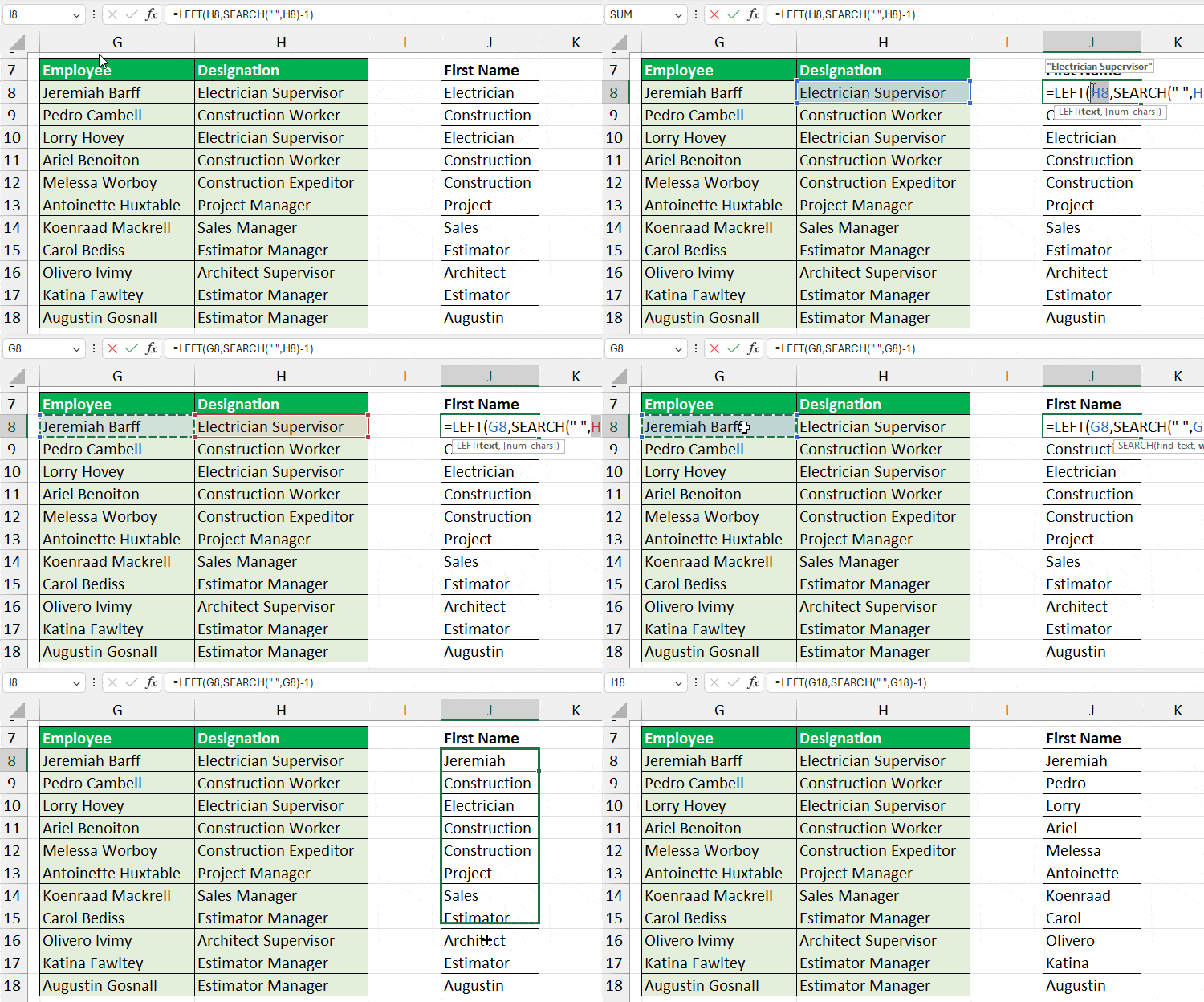
Remember, when using AutoFill to apply the formula to columns, you need to pay attention to the cell reference.

Know whether the Absolute Cell Reference or Relative Cell Reference is best for you.

Use the Find and Replace Menu

Find and Replace is another handy tool to quickly edit the column. You could use it to locate items within the cells and switch them with a different value.

For instance, change the numbers with a dot to a comma, find and remove a dash from the column, remove commas, time from date, and many more.

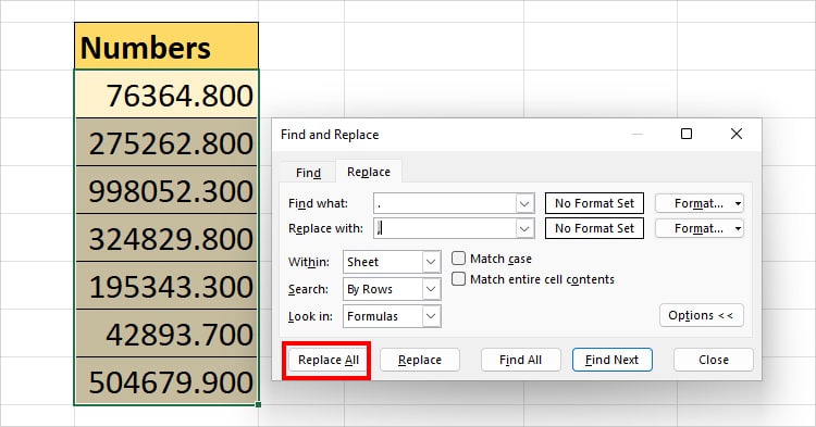
To do that, select the Columns. Then, enter Ctrl + H to bring up the Find and Replace menu.

Type the values in the Find what and Replace with field accordingly. Then, hit Replace All.

Use Paste Special

Paste Special is also best used to operate basic calculations like addition, subtraction, multiplication, and division.

With just the copy-and-paste command, you can perform quick operations and update the entire range at once.

Suppose, the values in Column A are multiplied by 2.4. But, now I want them to multiply by 3.8.

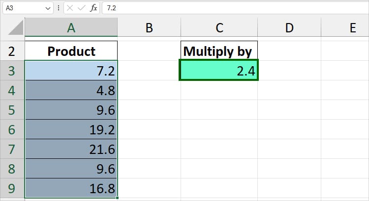
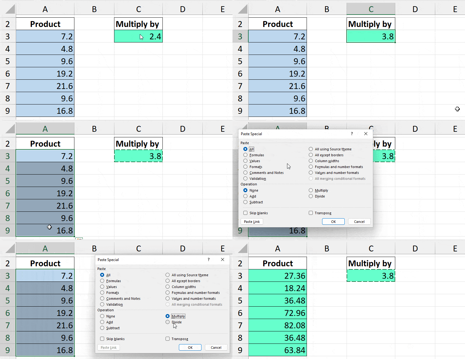
For that, enter a 3.8 number in a cell and copy it using the Ctrl + C. Now, select the Column A range. Right-click on it and choose the Paste Special menu.

On Paste Special, pick Multiply and hit OK. You’ll have the values updated for the entire Column A.

Format as Table

Whenever you add new information to the source data, you would have to re-enter the formula and include those cell references too. Especially, for lookup formulas like VLOOKUP, HLOOKUP, INDEX, XLOOKUP, OFFSET, etc.

While it’s easy to edit formulas, it can get monotonous over time.

So, instead, format the data as a table range. When you apply a Table, it uses Structured References instead of Explicit Cell References in the formula.

For example,

Structured References: =[@Sales] *[@[ Commission (%)]]/The table uses Column Headers.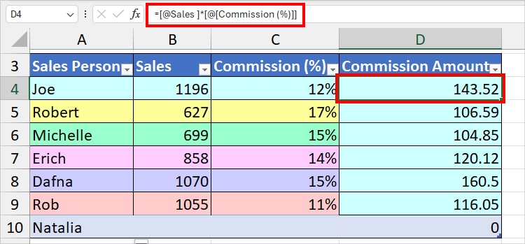

Explicit Cell References: =B4*C4/Cell references in a range of data.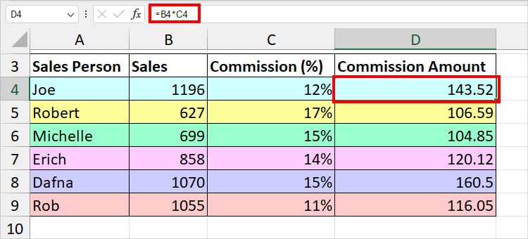

Therefore, even if you insert a new column or add a row, it won’t affect your formula columns.

Moreover, applying a Table format is also helpful when you need to auto-update the Excel Charts.

Use Whole Column Reference

If you want the column to auto-update before even entering the formula, set the whole column reference.

Suppose, I want to return all the texts from Column A in the uppercase.

Instead of passing down the selected reference in the formula, I will enter the entire Column A:A in the UPPER function. Then, extend the formula to remaining cells in Column B.

Formula: 

=UPPER(@A:A)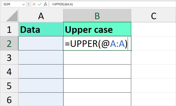

Now, when I enter data or paste values in Column A, I’ll have the uppercase text as output in Column B.

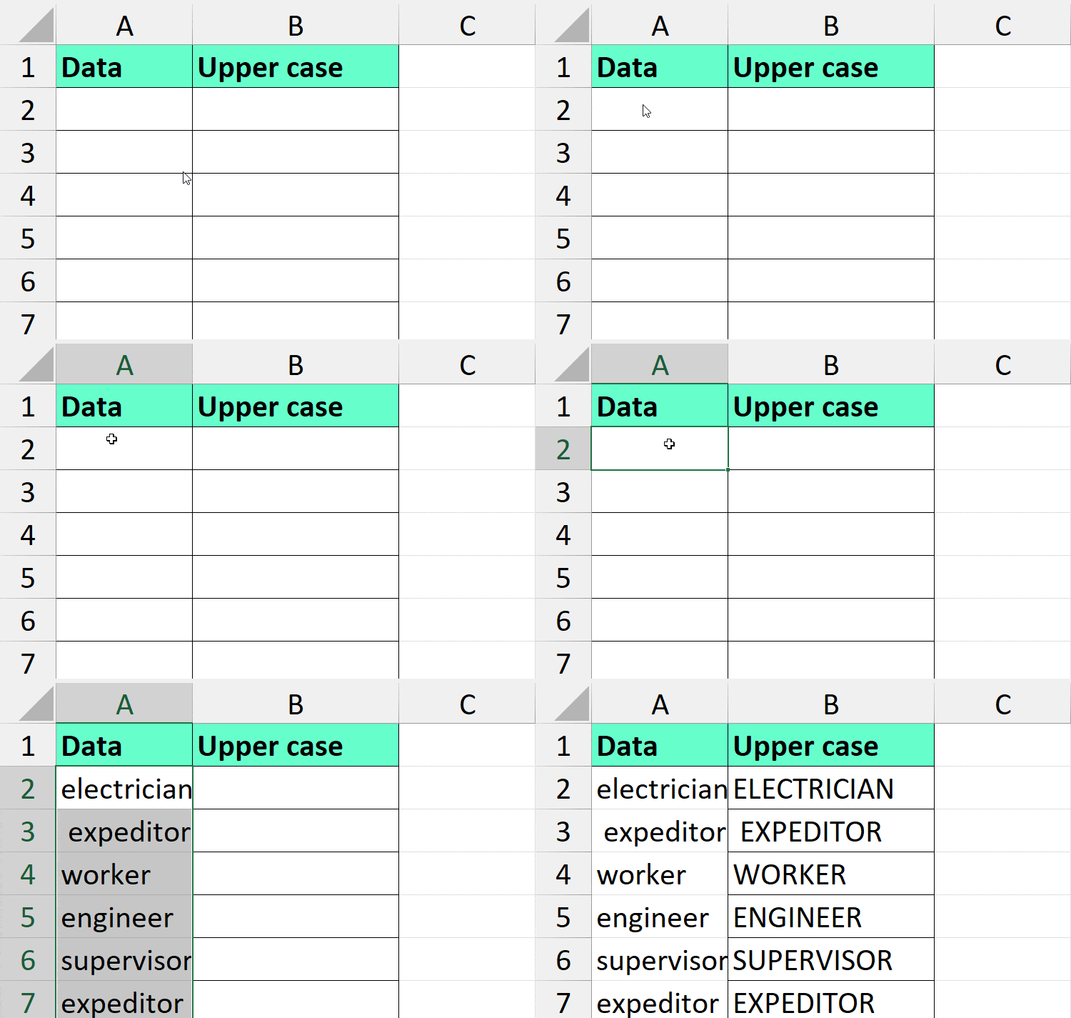
However, I wouldn’t recommend you use this in array and lookup functions.

Since the referencing takes the whole space, you won’t have the extra cells to spill output when you enter a formula in Column A. Eventually, you’ll have a #SPILL! Error in the cell.

Use Filter Tool

There can be instances when you may find the need to edit the column based on criteria.

To do that, you can add a filter tool in the Column. Use the Ctrl + Shift + L keyboard shortcut to turn on the filter.

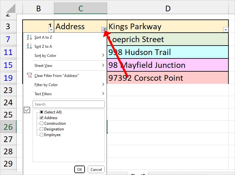
Click on the Filter button and display the rows you want to get rid of. Then, if needed, delete those filtered items.

Use Power Query

Next, the Power Query Editor tool is also Excel’s best feature to edit and transform your data.

You can easily load your data into the Power Query Editor window, make changes to your column, and import them back to your sheet.

In the Power Query Editor window, you’ll have the option to Delete Duplicates, Split Columns by different cases, Replace Values, Extract Values, Move Columns, Calculate Standard and Statistical Data, Add Custom Column, Duplicate Column, Use Conditional Column, and many more.

Moreover, you can also find the default missing menu in this Power Query like the Trim, Clean, lowercase, UPPERCASE, Capitalize each word, Prefix, Suffix, etc.

1. To use Power Query, go to the Data Tab.
2. From the Get & Transform Data, click on From Table/Range.
   
3. On the prompt, tick My Table has Headers and hit OK.
   
4. Now, on the Power Query Editor window, visit each Home, Transform, Add Column, and View Tab to edit your Column.
   
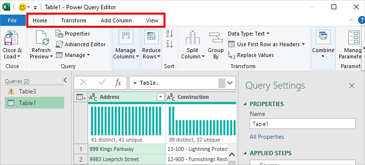
5. After you’re done, from Home Tab, hit Close & Load.
   

Use VLOOKUP Function

Let’s take for instance you need to update the present column based on the value of another sheet.

During that case, use the VLOOKUP between Sheets. Or, if needed, in different workbooks. It’s the best way to make your Column dynamic.

For example, you can link the cell of two sheets and extract data by entering the VLOOKUP formula. Here, I have drawn out the value from the MainSheet to my present worksheet.

Formula:

=VLOOKUP(A3, MainSheet!B3:E6, 4, FALSE)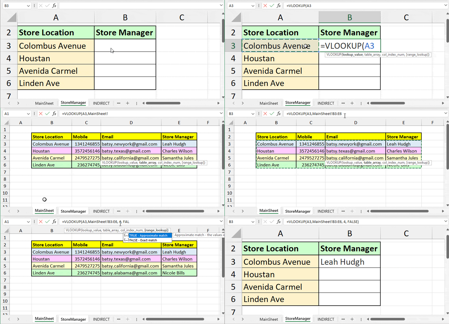

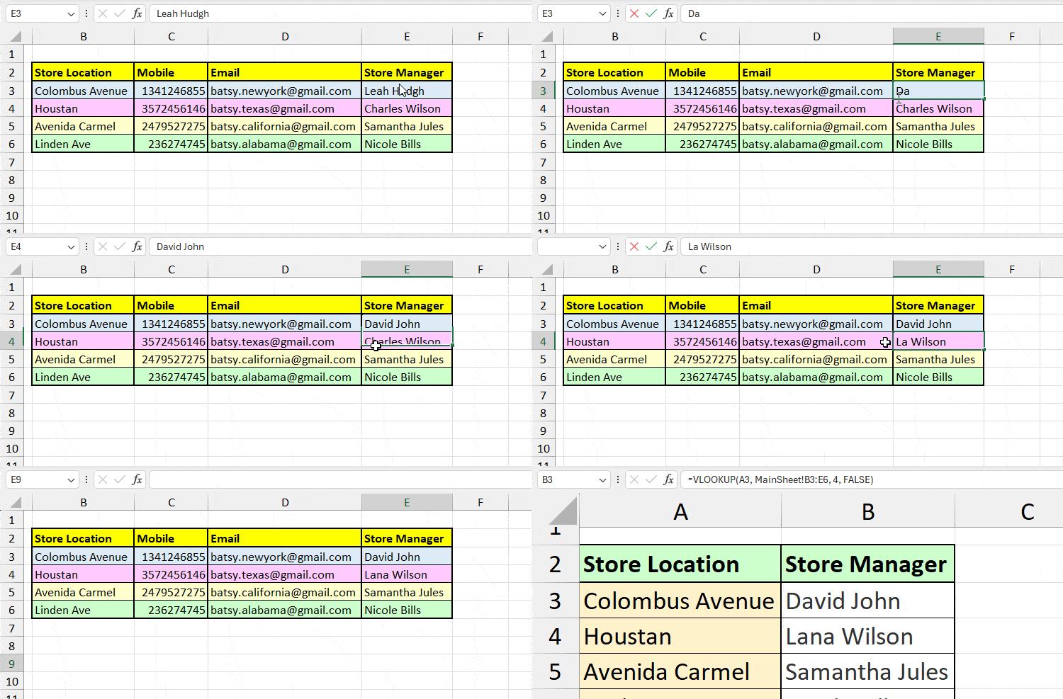
Above I got Leah Hudge as a result. Later, if I change the data in MainSheet, it’ll instantly update in StoreManager Sheet too.

Take a look at how the output automatically changed when I entered different names.

We have an in-depth guide on How to do a VLOOKUP between two sheets with examples.