In Excel, you may find the need to pinpoint duplicate values to remove, replace, highlight, filter, or count them.
Although there isn’t a dedicated feature to identify Duplicates like “Remove Duplicates,” we have several functions and features to do so.
Here, we will go through on how to use Conditional Formatting and functions like FILTER, COUNTIF, IF, etc., to find duplicates in 5 different cases.
Case 1: Find All Duplicates in a Sheet
While there are many ways to find all duplicates in Excel, I especially recommend you use Conditional Formatting for this.
This is because, with functions like COUNTIF, you will have a hard time tracking the cells that return TRUE for Duplicates – especially for big datasets.
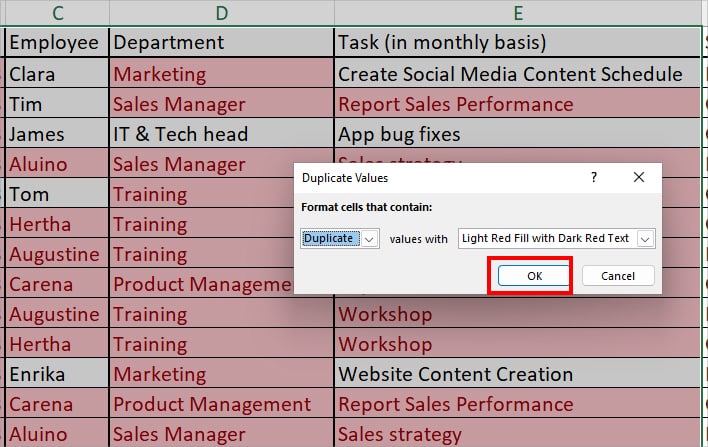
But, with Conditional formatting, you can quickly identify and highlight all duplicate entries.
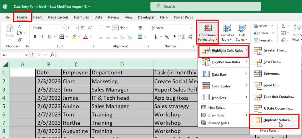
Simply, select cells of your Sheet. From your Home Tab, click Conditional Formatting > Highlight Cells Rules > Duplicate Values.
On Duplicate Values, pick a color and hit OK.
Case 2: Find Duplicates in Column
To know the Duplicates in the same column or different column, we will be using functions for this.
Example 1: Same Column
Suppose, you want to check and see the duplicate entries within the same column. To perform this, first, add a helper column.
Then, enter the COUNTIF formula as mentioned in the box. Remember, this formula will also take the first occurrences as duplicate values and mark them as TRUE.
=COUNTIF(C:C, C3) > 1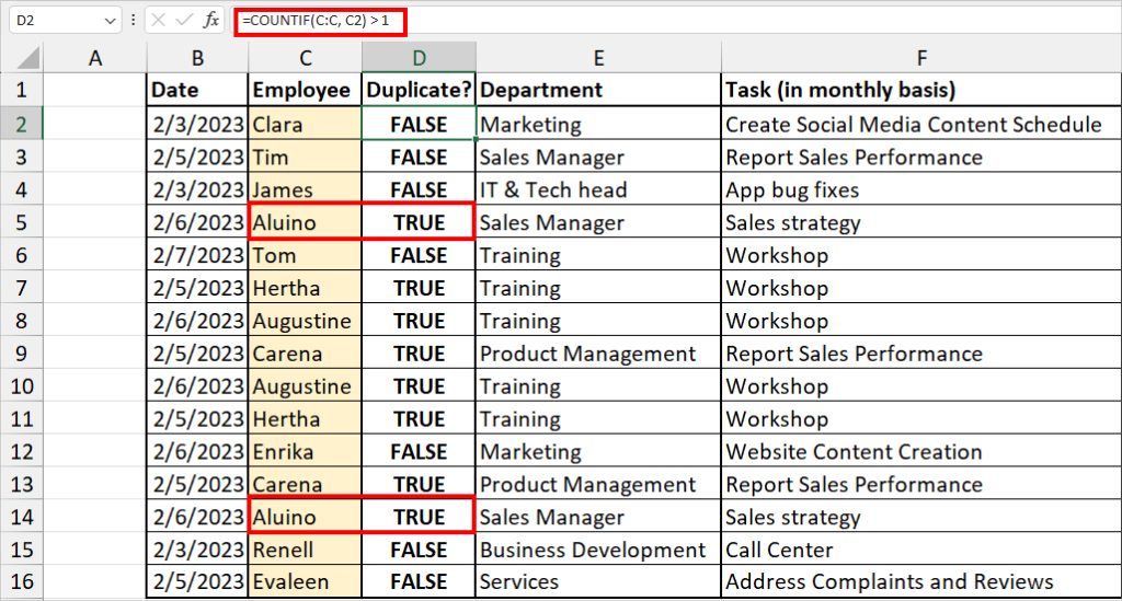
The COUNTIF formula above counts and returns the total number of cells with C2 (Clara) value from range C:C.
As we have specified greater than 1 criteria in the end, it returns TRUE for duplicates and FALSE when there is only a unique item.
In case you do not want to include the 1st occurrences of duplicate values, use this formula.
=IF(COUNTIF($C$2:$C2, C2) > 1, "Duplicate", "")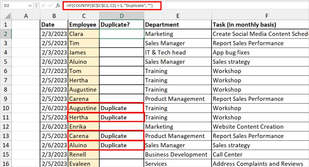
Example 2: Different Column
Next, to compare values between columns and identify the duplicates, we will use the UNIQUE and FILTER function nested together. It is the same as merging duplicates in Excel.
=UNIQUE(FILTER(B4:B10, COUNTIF(B4:B10, C4:C10)>0))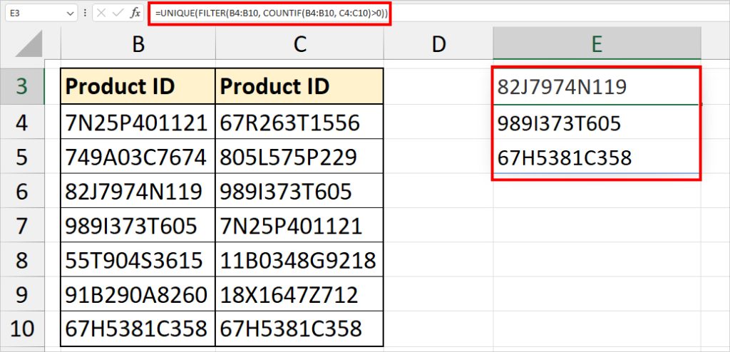
The COUNTIF formula first checks and returns the total number of repeated values in between both columns. Then, the FILTER function filters out and returns an array of duplicate values.
Finally, the UNIQUE function returns only the unique values from that filtered array.
Case 3: Find Duplicate Rows
You can also find the duplicate values based on rows in Excel. Firstly, combine all values of the column from a Row using the CONCAT function.
For that, enter =CONCAT(A4:C4). Then, copy the formula for the remaining cells.
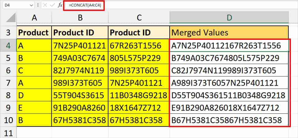
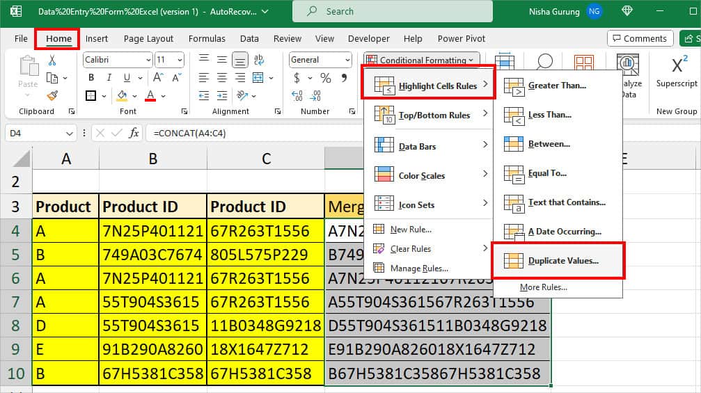
Now that we have values to check the duplicates, we will use Conditional Formatting.
On the Home Tab, navigate to Conditional Formatting > Highlight Cells Rules. Select Duplicate Values and hit OK.
Once you’re done, you can hide the merged values from the highlighted column. Select Column and enter Ctrl + 1. On the Number tab, click Custom. Enter ;;; in the Type field and hit OK.
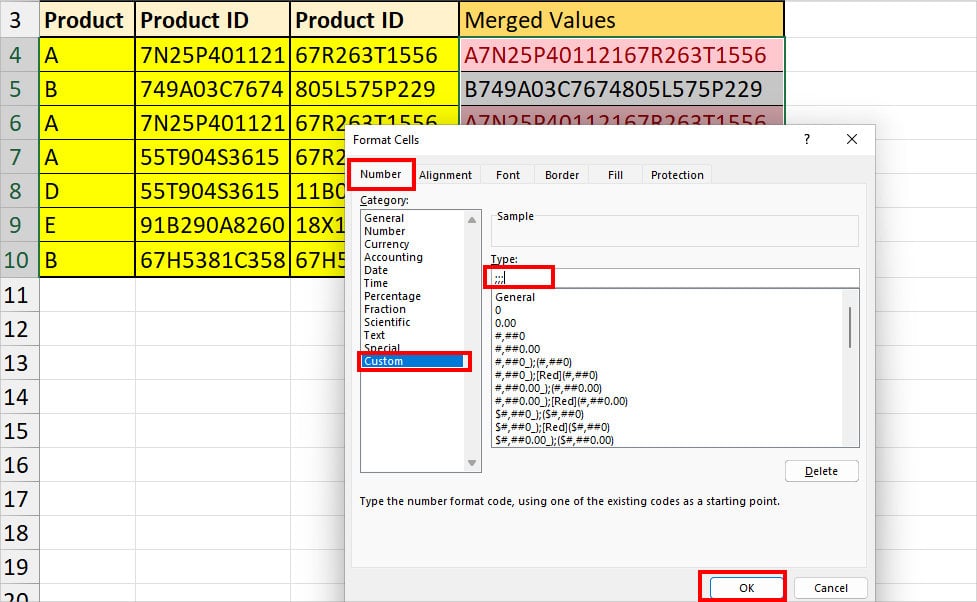
The numbers will be hidden now.
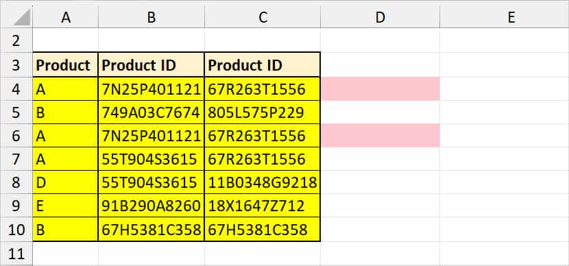
In case you want to delete duplicate rows based on one column, we have an article guide on how to do it.
Case 4: Find Case-Sensitive Duplicates
While searching for duplicates, Case-Sensitive is another thing you mustn’t miss out on.
In all the above cases, the formulas/features take both the lowercase (nisha) and Uppercase (NISHA) as duplicates in your spreadsheet.
But, let us consider them differently and find only the case-sensitive values as duplicates. Enter this formula in a new cell.
=IF(SUM((--EXACT($C$3:$C$11,C3)))<=1,"","Duplicate")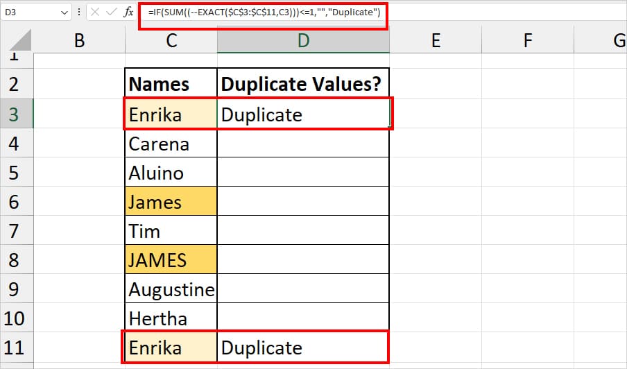
The formula returns “Duplicate” as a result in the cells where there are lowercase matches. Here, we got duplicates for “Enrika” only.
As seen in the picture, the formula ignored duplicate values for “James” and “JAMES.”
Case 5: Find Duplicates Across Sheets
So far, we learned how to find duplicates in a single spreadsheet. Now, let us check and highlight the duplicate values across sheets in a workbook.
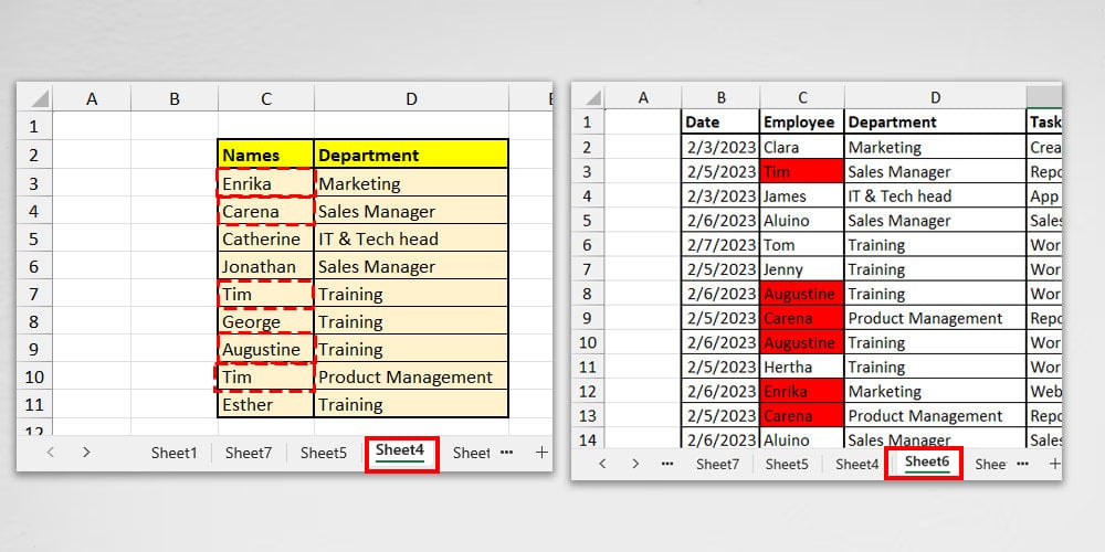
As an example, I will look for duplicate values in Sheet 6 and Sheet 4. Then, highlight duplicate cells.
- Firstly, on Sheet 6, Select ranges with duplicate values to highlight them.
- In the Home Tab, expand the Conditional Formatting menu > New Rule.
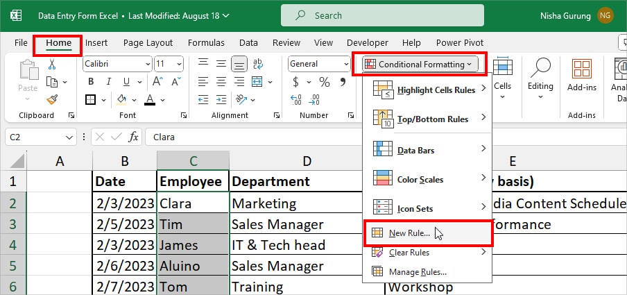
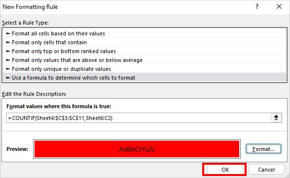
- Head to Use a formula to determine within cells to format menu and type the
=COUNTIF(Sheet4!$C$3:$C$11,Sheet6!C2)formula in the field.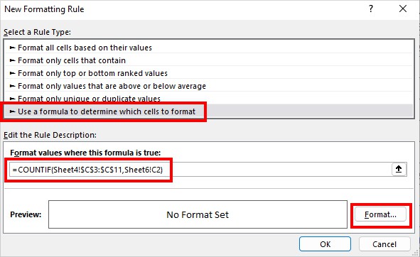
- Click Format. Then, select a Colour and hit OK.
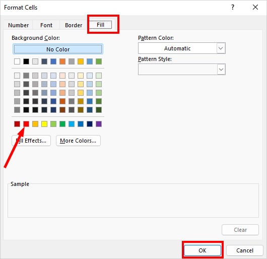
- Again, click OK.
- The formula will highlight the duplicate values of Sheet 6 that match with Sheet 4.
By now, you must’ve learned all the cases and methods to find duplicates. If you want to delete those duplicates, here’s our next article on “How to de-duplicate in Excel.”