How to Change Cell Color in Excel Based on Text Input

You can enter all sorts of data in Excel, including hierarchical ones. When dealing with such values, you may want to color code them using unique colors, or even create a heat map based on the values.

For such formatting, Excel has a dedicated tool called Conditional Formatting. You can use Conditional formatting to assign a color to specific values whether they’re text, numbers, or even special characters. What’s more, is that you can even create custom rules using Excel formulas to change the cell color.

Format Number Values Based on Inequalities

If you’re looking to format inequalities like greater than, less than, between, or equal, you can use the Highlight cell option in the Conditional Formatting tool. All you have to do is specify your number or range, and the formatting you wish to apply to the targeted cells.

1. Select your data range.
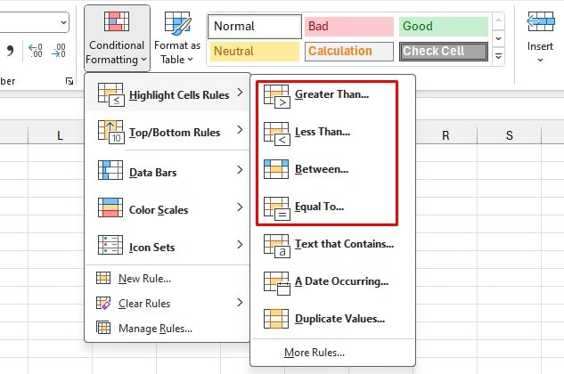
2. From the Home tab, select Conditional Formatting from the Styles section.
3. Hover your cursor over Highlight Cells Rules.
   

Highlight Numbers Greater Than

1. Choose Greater Than…
2. On the text box, enter the reference value. Conditional Formatting will format cells containing numbers greater than this value.
   
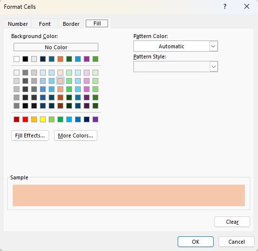
3. Next to with, specify a format. For more options, click Custom Format.
4. Click OK.

Highlight Numbers Lesser Than

5. Choose Less Than…
6. Enter than reference value. Excel will format cells containing numbers less than this value.
   
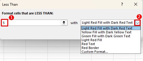
7. Next to with, specify a format. For more options, click Custom Format.
8. Click OK.

Highlight Numbers in Between

1. Select Between.
2. Enter the minimum value on the left and the maximum on the right.
   
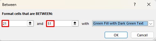
3. Next to with, enter the format.
4. Select OK.

Highlight Numbers Equal to

1. Click Equal To.
2. Enter the reference number.
   
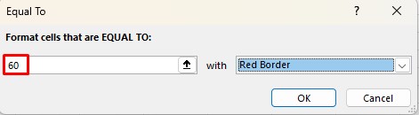
3. Choose your preferred formatting next to with.
4. Click OK.

Format Cells Containing a Text

You can also change the color of your cell based on whether it contains a specific text.

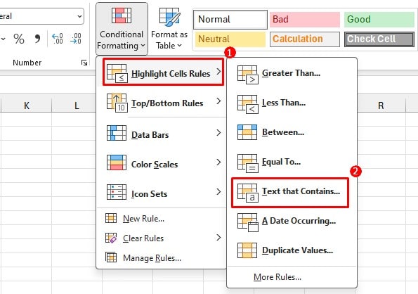
1. Go to Home.
2. Select Conditional Formatting from Styles.
3. Choose Highlight Cells Rules > Text that Contains.
   
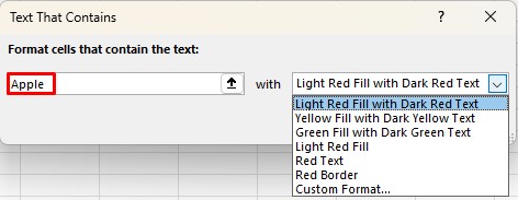
4. Enter your text in the text box.
5. Choose formatting next to with.
6. Click OK.

Format Cell Containing Dates

Using Conditional Formatting, you can format cells containing dates for yesterday, today, tomorrow, last week, and so on. Excel will your system’s date and time to format the cells, so make sure your device is running the correct date.

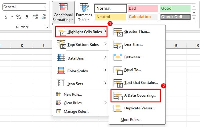
1. From the Home tab, select Conditional Formatting.
2. Choose Highlight Cells Rules > A Date Containing.
   
3. Select the left fly-out and choose a date.
4. Next to with, select a format.
   
5. Click OK. 

Format Duplicate or Unique Values

If your spreadsheet contains repeated values that you wish to locate, you can use Conditional Formatting to highlight such values. The tool will apply the set format to all values that have been repeated more than once on your spreadsheet.

Similarly, you can use the same interface to format cells containing Unique values.

1. Select Conditional Formatting from the Home tab.
2. Choose Highlight Cells Rules > Duplicate Values.
   
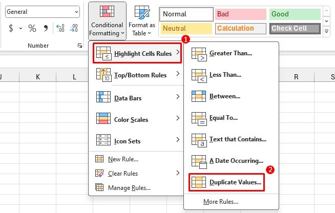
3. From the left fly-out, choose Duplicate to format repeated values else, select Unique.
4. Choose a formatting next to values with.
5. Click OK.

Change Cell Color Containing Top and Bottom Values

You can also apply the rule to format the cells containing top values in Excel. These rules contain formatting the top and bottom values, and the values that fall under the top 10% of your range. You can also change the percentile and item values from the conditional formatting interface.

1. Select your range.
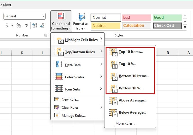
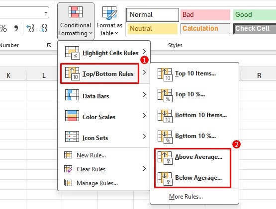
2. From Home, select Conditional Formatting.
3. Go to Top/Bottom Rules.
   

Format Cells Containing Top Items

1. Select Top 10 Items.
2. In the left text box, to increase the item number, use the up and down arrow keys.
   
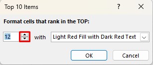
3. Next to with, choose a format.
4. Click OK.

Format Cells Containing Top Percentages

1. Choose Top 10%.
2. Increase or decrease the percentage value using the top and down arrow keys.
   
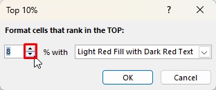
3. Select a cell format next to with.
4. Click OK.

Format Cells Containing Bottom Items

1. Select Bottom 10 Items.
2. If you wish to format cells containing a different bottom value, use the arrow keys to change the value from 10.
   
3. Next to with, choose a different format.
4. Click OK.

Format Cells Containing Bottom Percentages

1. Select Bottom 10%.
2. To change the percentile value, use the arrow keys.
   
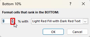
3. Change the cell formatting next to with.
4. Select OK.

Format Cells Containing Above or Below Average Values

Statistically, an average value refers to the sum of the given values divided by the number of items. If you’re analyzing a vast data set, you may want to look into which values are above and below the calculated average value.

For such analysis, you can use the Top/Bottom Conditional Formatting Rule.

1. Select the range containing your data set.
2. Head to Home > Conditional Formatting.
3. Choose Top/Bottom Rules.
4. Select either Above Average or Below Average.
   
5. Click on the fly-out to specify a format.
   
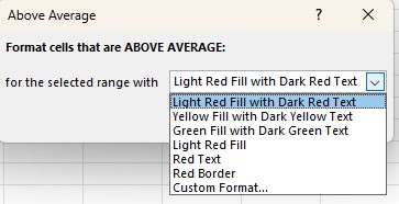
6. Click OK.

Create Heat Map

If your spreadsheet contains numerical data of the same kind, like temperature, you can create a heat map. Excel offers the option to create a heatmap using two or three-color scales. These colors can be both cool and warm-toned. Aside from a few library color palettes, you can customize your heatmap using your preferred colors.

1. From Home, select Conditional Formatting.
2. Choose Color Scales from the fly-out.
   
3. Select a color option to create a heatmap.
4. If you wish to customize the colors, select More Rules.
5. Under Edit the Rule Description, choose a Format Style.
6. Select the fly-outs in the Color section to pick colors for your heat map.
   
7. Choose OK.

Change Cell Color Using a Custom Formula

If you want to format your cells based on a specific formula, you can create a New Rule for conditional formatting. Let’s say you want to format cells based on their location. You can use the MOD and ROW functions to create a formula to highlight every few other rows.

1. Select Conditional Formatting from the Styles section in the Home ribbon.
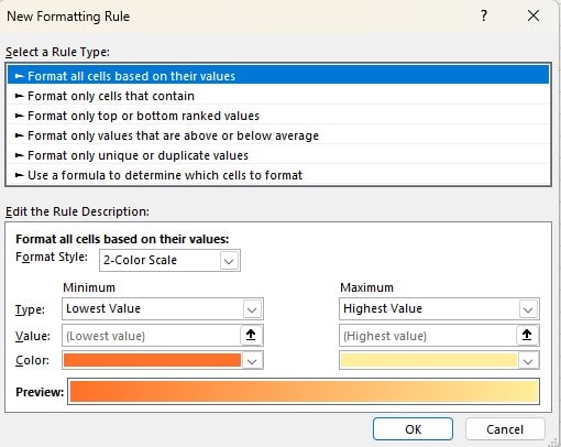
2. Click on New Rule.
   
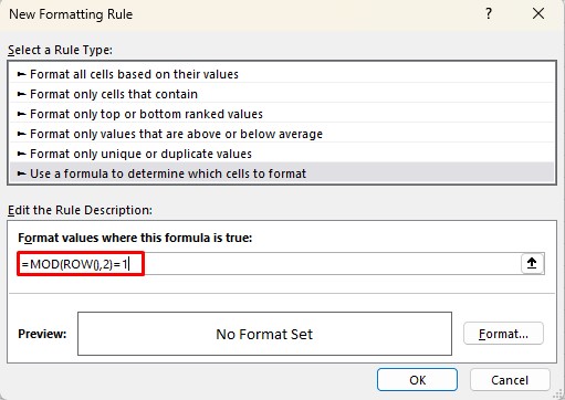
3. Under Select a Rule Type, choose Use a formula to determine which cells to format.
4. Enter your formula in the text box.
   
5. Click on the Format button to choose a format.
   
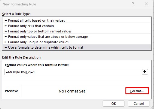
6. After previewing your format, click OK to confirm changes.