How to Delete Filtered Rows in Excel

Need to delete filtered rows in Excel?

Once you filter data in Excel, only the rows with applied criteria will be visible to you. So, simply select and right-click on those rows. Then, hit Delete Row and click OK to confirm.

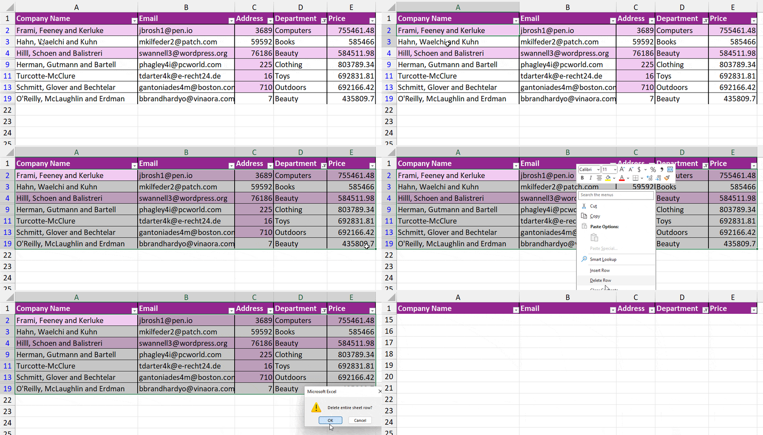
If your data is in a table format, select and right-click on Filtered Rows. Choose Delete > Entire Sheet Rows. This method is extremely useful and quick when you have a smaller dataset in the spreadsheet.

But, for larger rows, I have other efficient ways to delete Filtered Rows, which is by using Sort, VBA code, Power Query, Inspect Document Feature, etc.  

Using Sort and Delete Row

There can be situations where you have applied more than one filter to the row. If the values aren’t sorted, the filtered row to delete will be all over the place. 

Eventually, it can take hours to select and delete rows one by one, which hinders your productivity.

But, by using the Sort tool, you can separate all the filtered rows to delete in a contiguous range. It will remove only the filtered visible rows and keep the hidden ones intact. 

Example:

Suppose, I have filtered out rows with Electronics, Beauty, and Baby departments. I need to delete all the rows with Beauty.

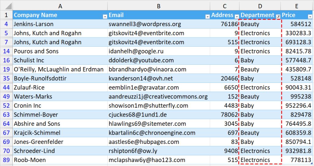
1. Firstly, select any cell in your Column Header. 
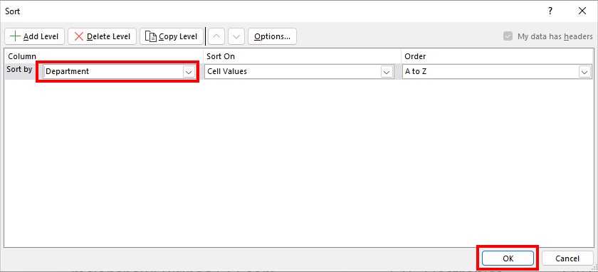
2. On the Data Tab, click on the Sort menu.
   
3. On the Sort window, hover over the Sort by menu. Expand the Drop-down and choose Heading. Here, I picked Department.
   
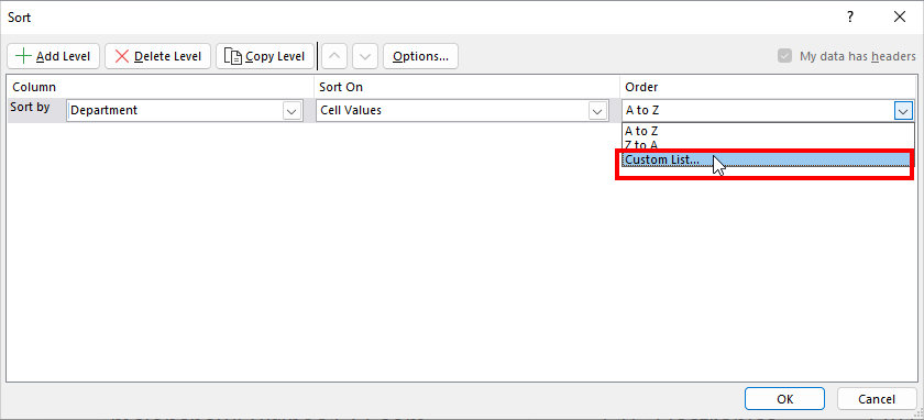
4. Next, on Order, select Custom List.
   
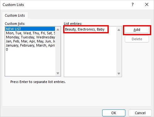
5. Click the Add button. Then, on List entries, enter the Order you want to Sort Values in. Then, hit OK. For example, I typed in Beauty, Electronics, and Baby.
   
6. Click OK.
   
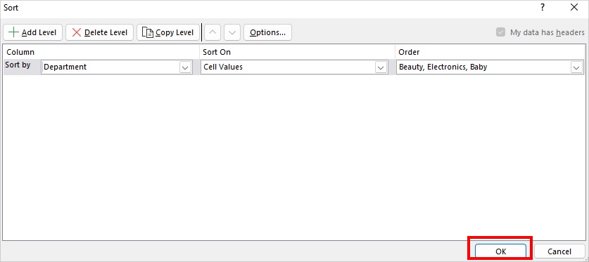
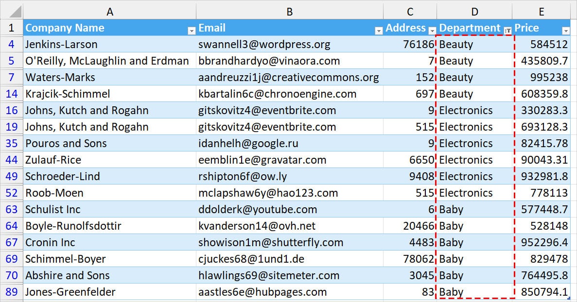
7. Now, you’ll have the filtered rows as specified in the custom sort.
   
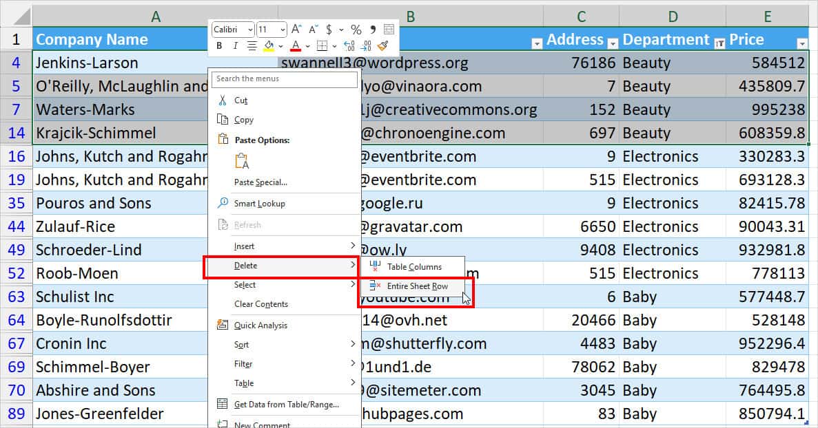
8. Select those rows. Right-click and pick Delete > Entire Sheet Row.
   

Using Power Query

If you need to delete huge chunks of filtered rows like 35,000 or 40,000 rows, your Excel might crash when doing it at once.

Even if you manage to delete rows in a batch like 5000 rows at a time, it’ll take forever to accomplish your task with this speed. 

Instead, as a workaround, you can use the Power Query Tool. Here, we won’t be eliminating the filtered data. 

But, we will load the data into Power Query, filter rows that you do not want to delete, and import only those visible data into a new worksheet. Later, you can get rid of your original data if you want.

You can also opt for this method when you’re importing external files like CSV, JSON, XML, etc into Excel. Perform these steps before loading a file into a sheet in the Power Query Editor. 

1. Select your data and head to the Data Tab. 
2. Click on From Table/Range. Click OK on the prompt box.
   
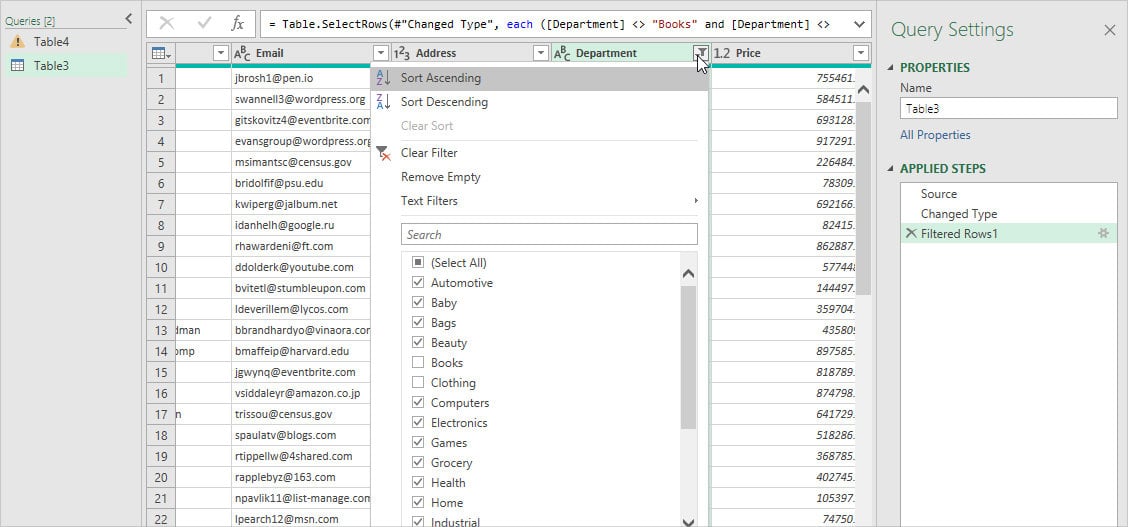
3. On the Power Query Editor window, Filter the Rows the same way you do in the Sheet. On the column, expand the Filter button. Tick the boxes for values to show and hit OK.
   
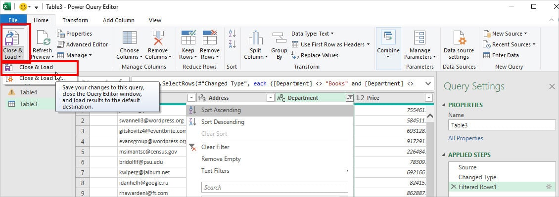
4. On the Home Tab, choose Close & Load. Again, pick Close & Load.
   

Using Inspect Document Feature

Let’s assume, you have hidden filtered rows from your data and you want to delete them. Rather than unhiding and eliminating rows, we will use the Inspect Document Feature to quickly perform this.

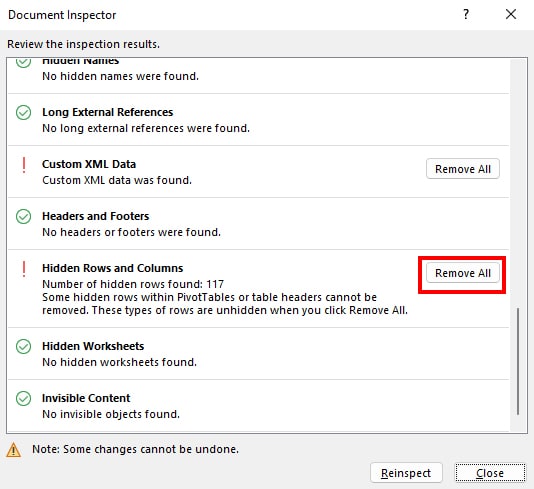
Keep in mind that once you hit Remove All, Excel won’t send you another confirmation prompt. The hidden rows/columns will be deleted immediately. 

Before you begin, in the Filter tool, show all the rows you want to keep in the Worksheet. If you filter out them, the tool will consider them as a hidden row and remove them too.

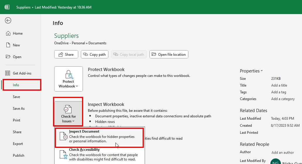
1. From the File Tab, click on the Info menu.
2. Expand Check for Issues > Inspect Document.
   
3. On the prompt box, choose Yes.
   
4. Click Inspect.
   
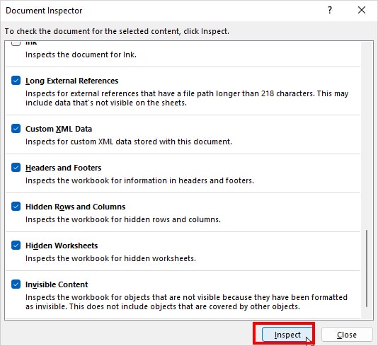
5. Now, locate the Hidden Rows and Columns menu and hit the Remove All button.
   

Using VBA Code

For users who need to remove the filtered rows more often, I recommend you use the VBA code. 

Here, I have given the code to delete the filtered rows which are both visible and hidden. You can simply specify the variables in the VBA code as per your data and hit Run. 

To use VBA, make sure there is a Developer Tab in your worksheet. If necessary, add the Developer Tab. 

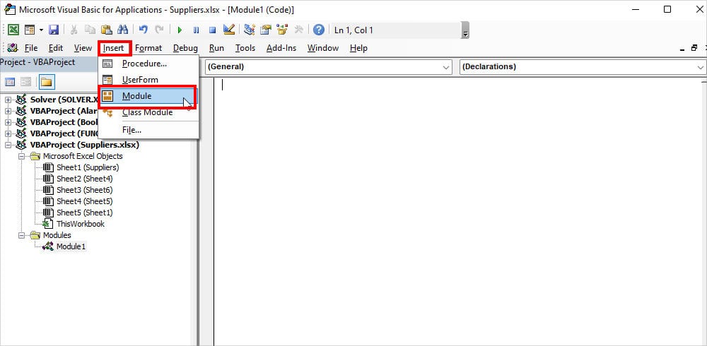
First, select the cell ranges. For the VBA window, enter the Alt + F11 shortcut key. Click Insert > Module. Then, Copy and paste either of the given code.

Delete Filtered Visible Row

Here, enter the value for “Filtered Column Number” and “Filtered Value to Delete.” For example, to delete the filtered rows with Computers, my field will be 4 as it is in the 4th column. Criteria 1 is “Computers.“

Sub DeleteFilteredRows()
Dim Rng As Range
Set Rng = Selection
Rng.AutoFilter Field:= “Filtered Column Number”, Criteria1:="Filtered Value to Delete"
Rng.Offset(1, 0).SpecialCells(xlCellTypeVisible).EntireRow.Delete
ActiveSheet.AutoFilterMode = False
End Sub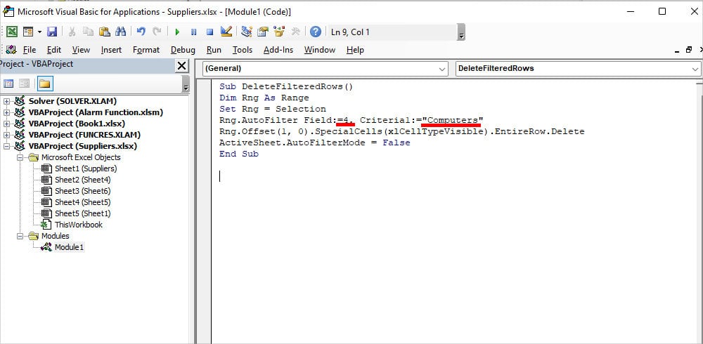

Delete Filtered Hidden Rows

This time it’s the opposite. Here, the code keeps the displayed Filtered ranges and deletes the unfiltered or hidden ones.

Again, just like above, specify the “Column Number” and “Filtered Value to Keep” as per your data. But remember, you are keeping these values on your sheet.

You can specify R.AutoFilter Field:="Column Number", Criteria1:="Filtered Value to Keep" as many rows as you want to show in the code.

As an example, I have chosen to display only 3 rows in the criteria and delete the rest of them.

Sub DeleteHiddenFilteredRows()
Dim myU As Range
Dim myR As Range
Dim R As Range
Set R = Selection
R.AutoFilter Field:="Column Number", Criteria1:="Filtered Value to Keep"
R.AutoFilter Field:="Column Number", Criteria1:="Filtered Value to Keep"
R.AutoFilter Field:="Column Number", Criteria1:="Filtered Value to Keep"
For Each myR In R.Rows
 If myR.Hidden Then
 If Not myU Is Nothing Then
 Set myU = Union(myU, myR)
 Else: Set myU = myR
 End If
 End If
Next
myU.Delete
ActiveSheet.AutoFilterMode = False
End Sub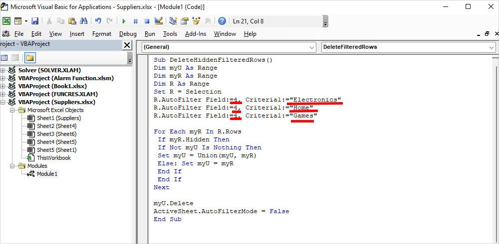

Finally, Press F5 to Run the VBA code.