During Data Entry in Excel, most of the time, we do not have the names in alphabetical order. So, when you need to pinpoint a specific value, you might waste your time finding it.
But, if you just sort those data in A to Z or Z to A order, locating values will be a piece of cake! It’ll make your data more clean, organized, and professional.
Before You Begin
As you may encounter several issues when sorting names in Excel, follow these tips to be on the safe side.
- Check and Delete Blank Cells
- Unhide the Hidden Rows and Columns
- Trim Unnecessary Spaces from the Values
- Unmerge Merged Cells
Alphabetize Columns in Excel
Using A to Z or Z to A Sort button
The simplest and fastest approach to alphabetizing Columns is using the Sort button/keyboard shortcut. It will rearrange the columns in the specified order and keep the rest of the rows as it is.
Select the data and press the given Ribbon Shortcut.
Sort A to Z: Alt + A + SA
Sort Z to A: Alt + A + SD
Or, you could also do this from the Ribbon. On your spreadsheet, click on a Cell to alphabetize the column. Then, on the Data tab, hover over Sort & Filter section and click any one of the given buttons.
- A-Z Button: Categorize texts in Ascending Order.
- Z-A Button: Arrange texts in Descending Order.
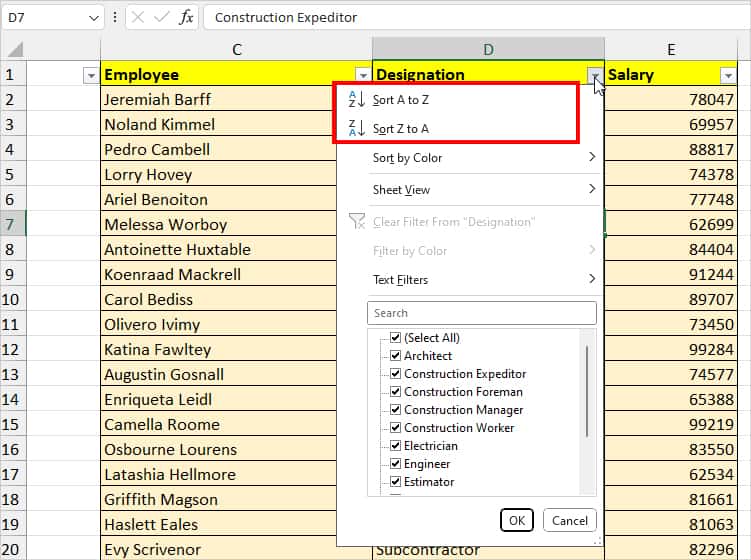
Using Filter Tool
Next, you can change the order of alphabets using the Filter Tool. Again, the process is pretty much the same as above. Excel sorts a single column and keeps other data intact.
Click on any cell. Then, press the Ctrl + Shift + L shortcut to enable the Filter.
Now, expand the Filter button next to the Column header and choose Sort A to Z or Sort Z to A.
Using SORT Function
Excel has a SORT function to reorder the values in an ascending or descending manner.
While it could be used solely to return the sorted order, it is especially helpful to calculate and reorder items at the same time in practical life.
| Function | Syntax | Arguments |
| SORT | =SORT(array, [sort_index], [sort_order], [by_col]) | array: range you want to reorder Sort_index: row or column number to sort Sort_order: Specify how you want to sort 1: Ascending Order -1: Descending Order [by_col]: Enter Boolean to define your sort direction. TRUE: Rearrange by Column FALSE: Reorder by Row |
As an example, let me use the SORT and FILTER functions together.
Suppose, I want to filter and extract the names whose salary is less than 70,000. Also, I want the Answers to be in A to Z order.
Now, to achieve that result, I constructed this formula.
=SORT(FILTER(C2:E15, E2:E15 <G4, ""), 1, 1)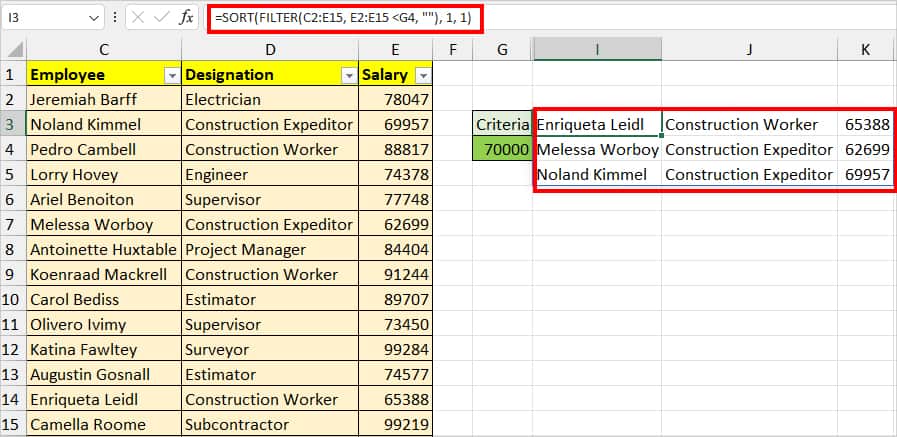
As specified in the formula, we got filtered names and numbers that are in ascending order.
Remember, as both functions are Array formulas, it will lead to #SPILL! Error in case there’s no empty cell to spill the outcomes.
If you’ve come across such an instance, check out our article on “How to correct #SPILL! Error in Excel?”
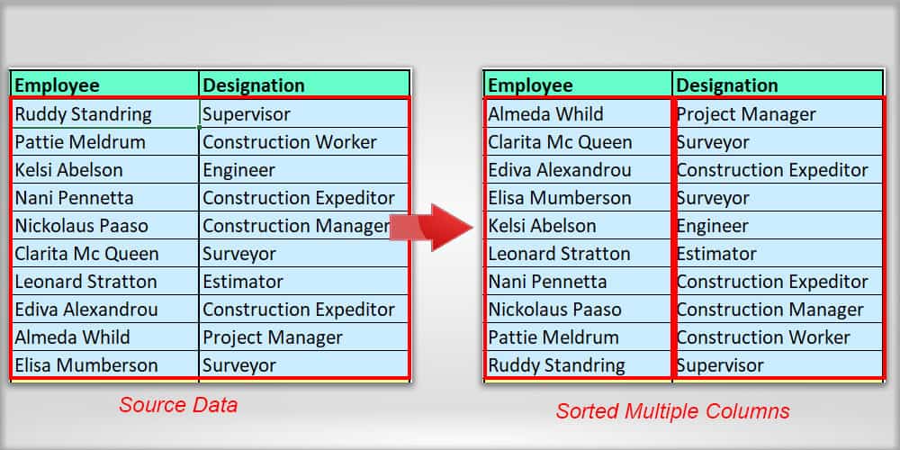
Alphabetize Multiple Columns
The above two methods do not sort the multiple columns. So, if you want to rearrange more than one column at once, Sort Button is the best.
Here, we will also learn how to reorder the values in our own custom format or arrange the case-sensitive text strings.
- First, click on Cell.
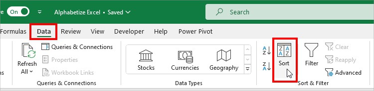
- From the Data Tab, click on the Sort button.
- On the Sort Window, expand the drop-down for Sort by and pick a Column Header.
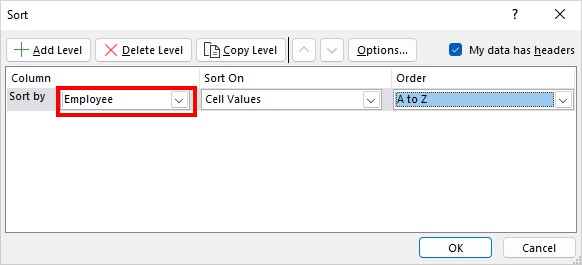
- Then, on Order, pick any one option.
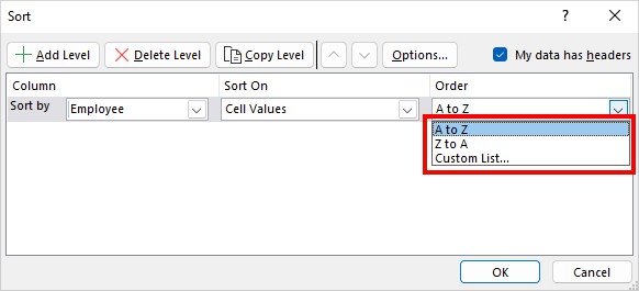
- Z to A: Reorder data in the Descending Order.
- A to Z: Rearrange data in Ascending Order.
- Custom List: Arrange text strings in Custom Order. If you pick this type the order in the List entries and hit OK.
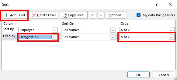
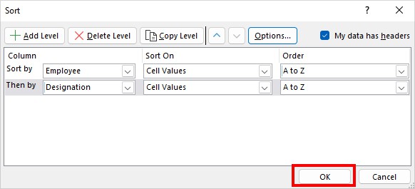
- Now, to add more columns, click Add Level. After that, in Then by, choose Column and Order just like in steps 3 and 4.
- For Case Sensitive reorder, hit the Options menu and tick the Case sensitive box. Click OK.
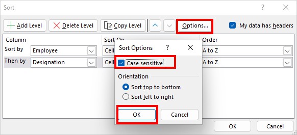
- When you’re done hit OK.
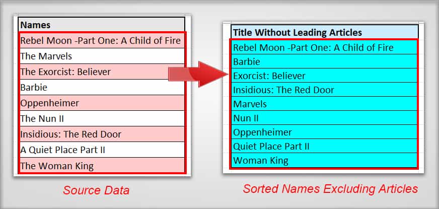
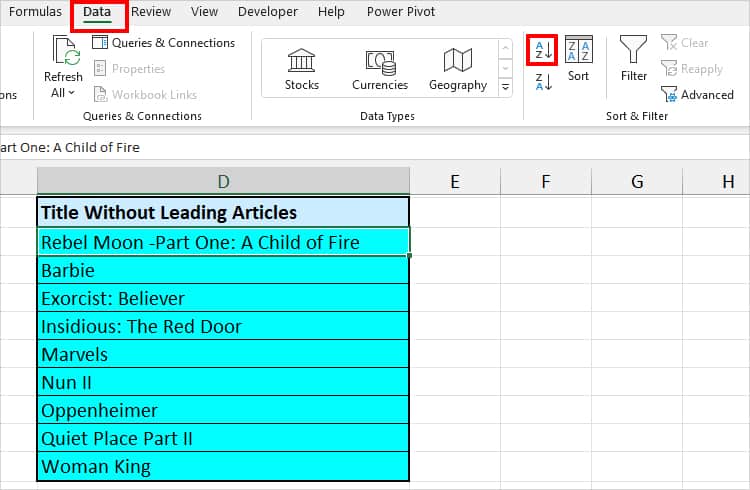
Alphabetize Columns Excluding Articles
With the Sort button, it’ll take articles such as The, A, and An as texts and reorder accordingly. But, if you want to exclude them and start the sort from the actual proper noun, we have a formula to do so.
Example:
I have listed down the Movies I watched this year which are in random order. I want to sort them in an A to Z order.
First of all, I will extract and make a new title for the movies without the articles. This is the formula.
=IF(IFERROR(FIND("The",B3,1)=1,0),SUBSTITUTE(B3,"The","",1),IF(IFERROR(FIND("A ",B3,1)=1,0),SUBSTITUTE(B3,"A ","",1),B3))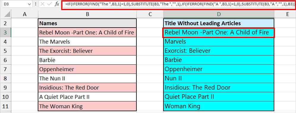
Then, copy-paste the result Column as value only. After that, head to Data tab and click on A to Z or Z to A button.
Sort Alphabetically By Last Name
Suppose, you have lists of Full Names and you want to alphabetically sort the values by the Last Name like in the given image.
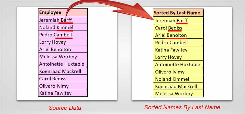
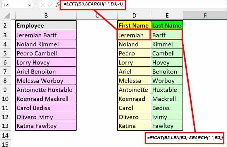
To do that, we will first extract the First and Last Names in Separate columns. Then, fill the rest of the columns using the Flash Fill.
| Example | Formula | Description |
| Extract First Name | =LEFT(B3,SEARCH(” “,B3)-1) | Here, with the SEARCH function, we are looking for values before space. Then, returning the texts using the LEFT function. |
| Extract Last Name | =RIGHT(B3,LEN(B3)-SEARCH(” “,B3)) | Here, with RIGHT, LEN, and SEARCH functions, we returned the Text Strings after the space from the right side. So, we got the Last Name. |
Once we have our data ready, we will concat the last name and first name. This time let us separate the names by a comma.
Formula:
=E3&", "&D3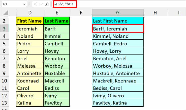
Now, copy down the formula. Then, select the Range and Copy-Paste as Value Only.
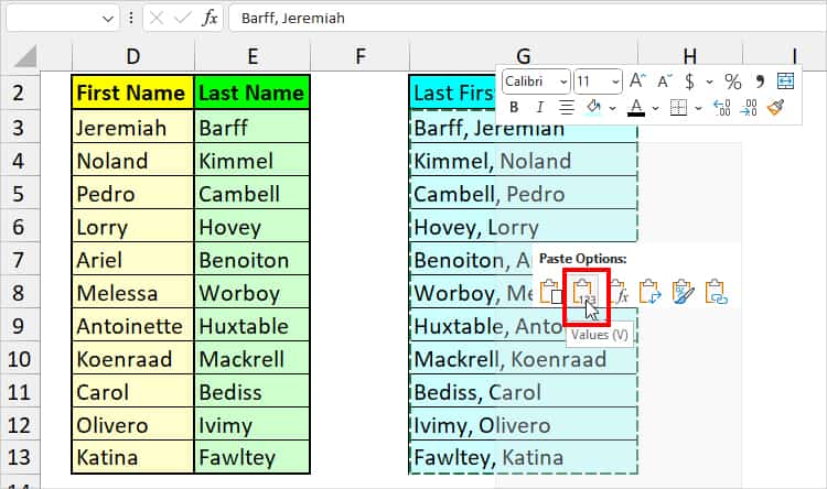
After that, from the Data Tab, click A to Z or Z to A Sort button.
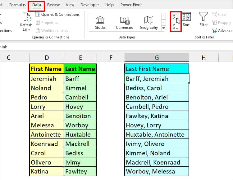
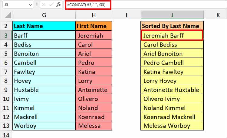
Finally, you can either leave the names as it is. Or, again, split the sorted first and last names using Text to Columns. Then, concat values again to format it as the original source.
Alphabetize Row in Excel
Up to this point, we have discussed how to sort the columns. Now, let us see the steps to alphabetize Row.
- Select Range to Sort.
- Navigate to the Data Tab and hit Sort.
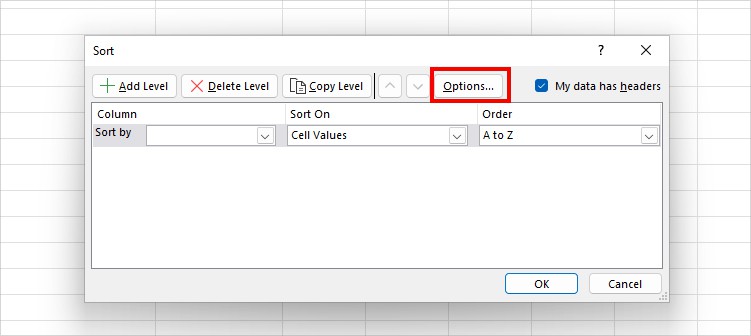
- On the Sort window, choose Options.
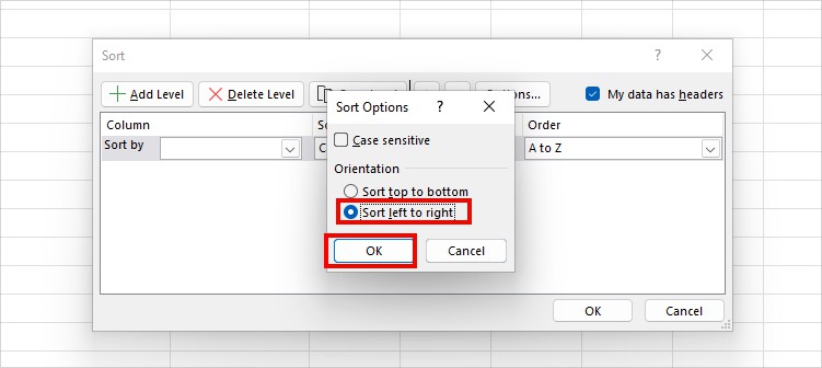
- Now, in the Sort Options box, pick Sort left to right. Then, click OK.
- Expand the drop-down lists for Sort by and choose a Row. Pick an Order.
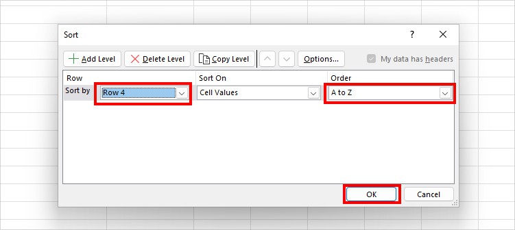
- Finally, click OK.
Alphabetize Rows Based on One Row
Next, we will be using Power Query to rearrange the values in Ascending or Descending order.
Now, you must be wondering why use such an advanced tool just to sort the Names?
Well, Power Query has all the required features and tools to transform your Data in any way you want.
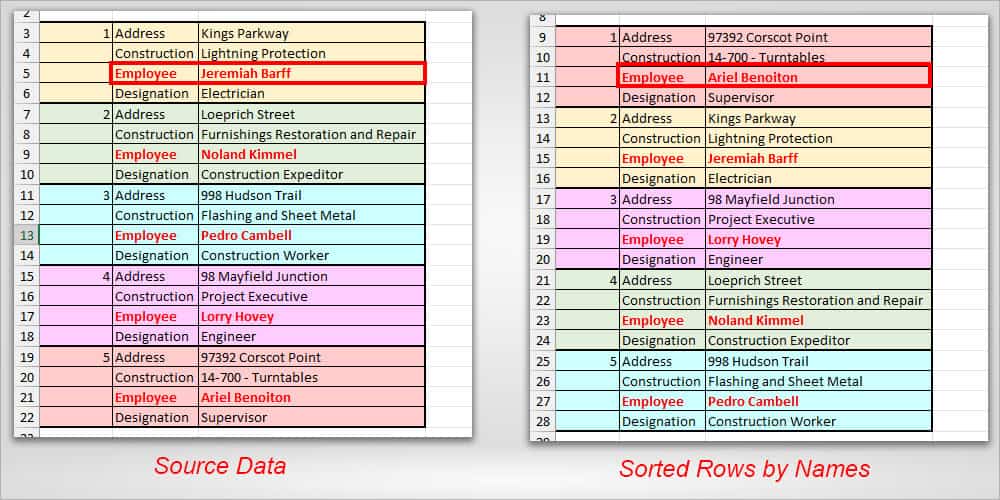
For Instance, here’s my data, and I want to sort the rows based on the Names alphabetically. I also don’t want the remaining categories to change. The only way to edit my values is using the Power Query.
- First, Select all values.
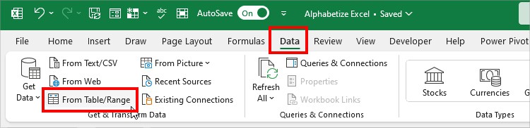
- From Data Tab, click From Table/Range.
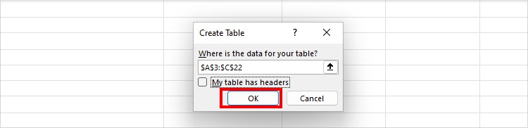
- When prompted, click OK.
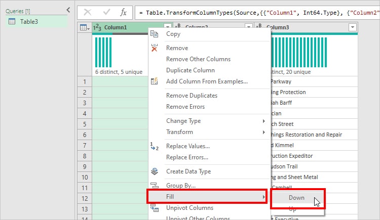
- Now, since my first column (Column1) has an empty cell, I will fill that first. Right-click on the Column1 Header > Fill > Down.
- Click on the Column2 Header (Category column). Go to the Transform tab and choose Pivot Column.
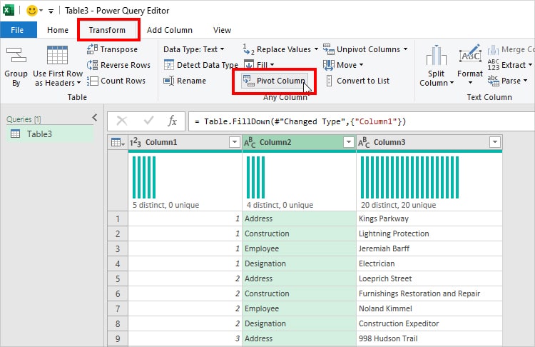
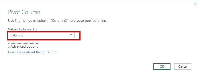
- On the Pivot Column window, select a Names Column.
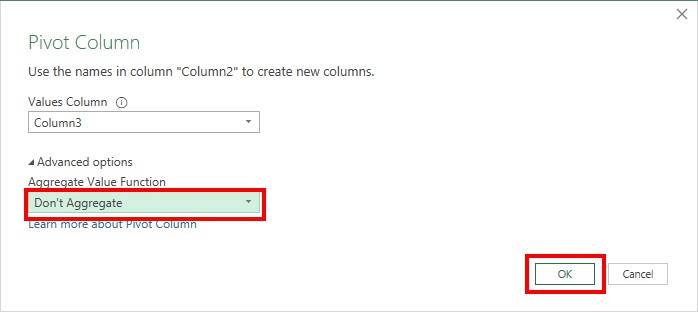
- Expand Advanced Options menu. Set the Aggregate Value Function to Don’t Aggregate and click OK.
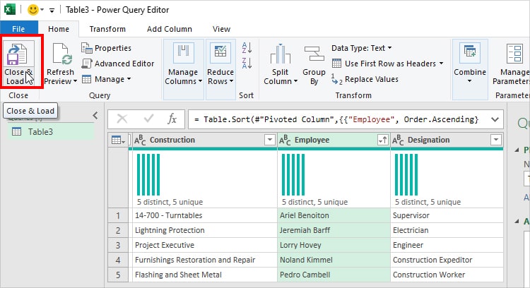
- Now, select the Employee Column. From the Home Tab, click on A to Z or Z to A Sort button.
- Finally, hit Close & Load in the Home Tab.
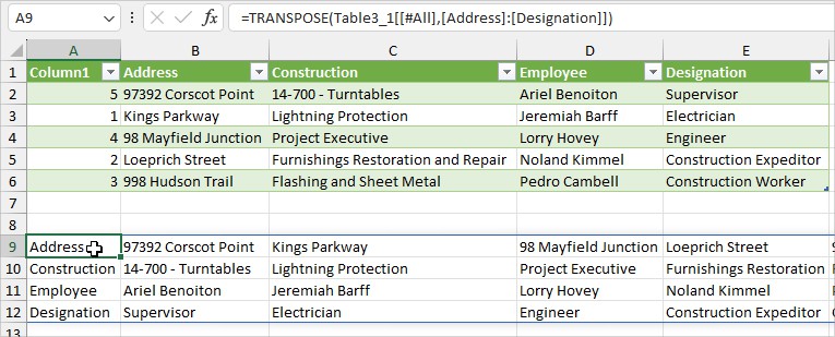
- You’ll have results in the Column Format. Use Transpose to Switch Rows and Columns.
Alphabetically Sort Only Selected Rows
Suppose, you want to sort only selected rows in Excel. Since there are no such built-in features, we can run a VBA code to achieve this.
Also, here, I have constructed the Code that will also prompt you to choose a Column to sort by and the Order(A to Z) or (Z to A).
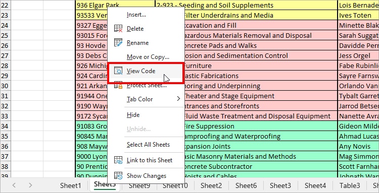
- Select the Rows you wish to sort.
- Right-click on the Sheet Name > View Code.
- On the Module, copy this code and paste it.
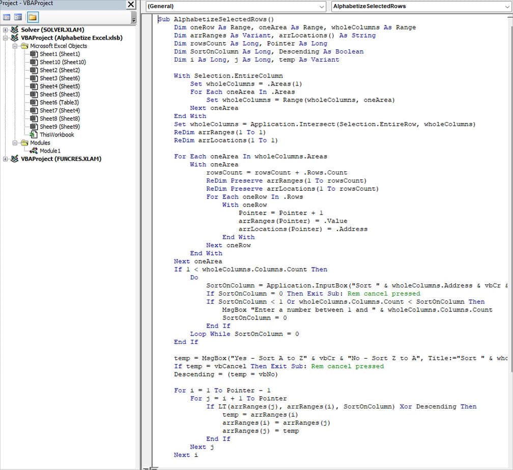
Sub AlphabetizeSelectedRows()
Dim oneRow As Range, oneArea As Range, wholeColumns As Range
Dim arrRanges As Variant, arrLocations() As String
Dim rowsCount As Long, Pointer As Long
Dim SortOnColumn As Long, Descending As Boolean
Dim i As Long, j As Long, temp As Variant
With Selection.EntireColumn
Set wholeColumns = .Areas(1)
For Each oneArea In .Areas
Set wholeColumns = Range(wholeColumns, oneArea)
Next oneArea
End With
Set wholeColumns = Application.Intersect(Selection.EntireRow, wholeColumns)
ReDim arrRanges(1 To 1)
ReDim arrLocations(1 To 1)
For Each oneArea In wholeColumns.Areas
With oneArea
rowsCount = rowsCount + .Rows.Count
ReDim Preserve arrRanges(1 To rowsCount)
ReDim Preserve arrLocations(1 To rowsCount)
For Each oneRow In .Rows
With oneRow
Pointer = Pointer + 1
arrRanges(Pointer) = .Value
arrLocations(Pointer) = .Address
End With
Next oneRow
End With
Next oneArea
If 1 < wholeColumns.Columns.Count Then
Do
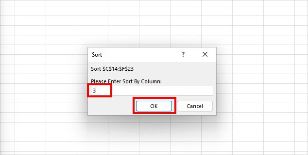
SortOnColumn = Application.InputBox("Sort " & wholeColumns.Address & vbCr & vbCr & "Please Enter Sort By Column:", Title:="Sort ", Default:=1, Type:=1)
If SortOnColumn = 0 Then Exit Sub: Rem cancel pressed
If SortOnColumn < 1 Or wholeColumns.Columns.Count < SortOnColumn Then
MsgBox "Enter a number between 1 and " & wholeColumns.Columns.Count
SortOnColumn = 0
End If
Loop While SortOnColumn = 0
End If
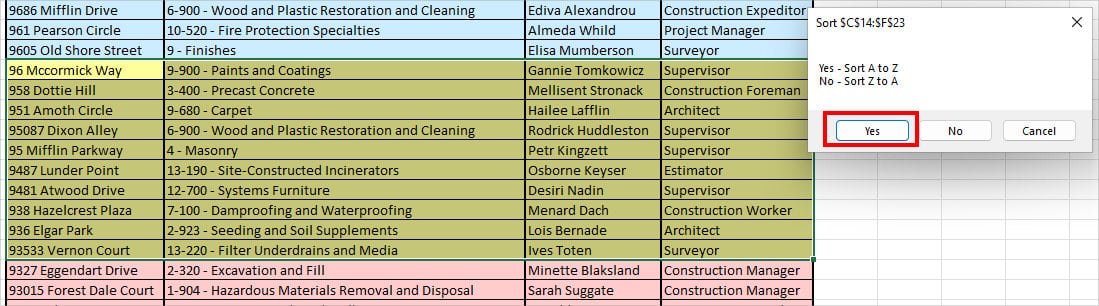
temp = MsgBox("Yes - Sort A to Z" & vbCr & "No - Sort Z to A", Title:="Sort " & wholeColumns.Address, Buttons:=vbYesNoCancel)
If temp = vbCancel Then Exit Sub: Rem cancel pressed
Descending = (temp = vbNo)
For i = 1 To Pointer - 1
For j = i + 1 To Pointer
If LT(arrRanges(j), arrRanges(i), SortOnColumn) Xor Descending Then
temp = arrRanges(i)
arrRanges(i) = arrRanges(j)
arrRanges(j) = temp
End If
Next j
Next i
For i = 1 To Pointer
Range(arrLocations(i)).Value = arrRanges(i)
Next i
End Sub
Function LT(a As Variant, b As Variant, sortColumn As Long) As Boolean
If sortColumn = 0 Then
LT = (a < b)
Else
LT = (a(1, sortColumn) < b(1, sortColumn))
End If
End Function
- Press F5 to Run.
- Then, on Please Enter Sort By Column dialogue box, type your Column Number and click OK.
- Again, on Sort Window, choose Yes for A to Z order and No for Z to A order.
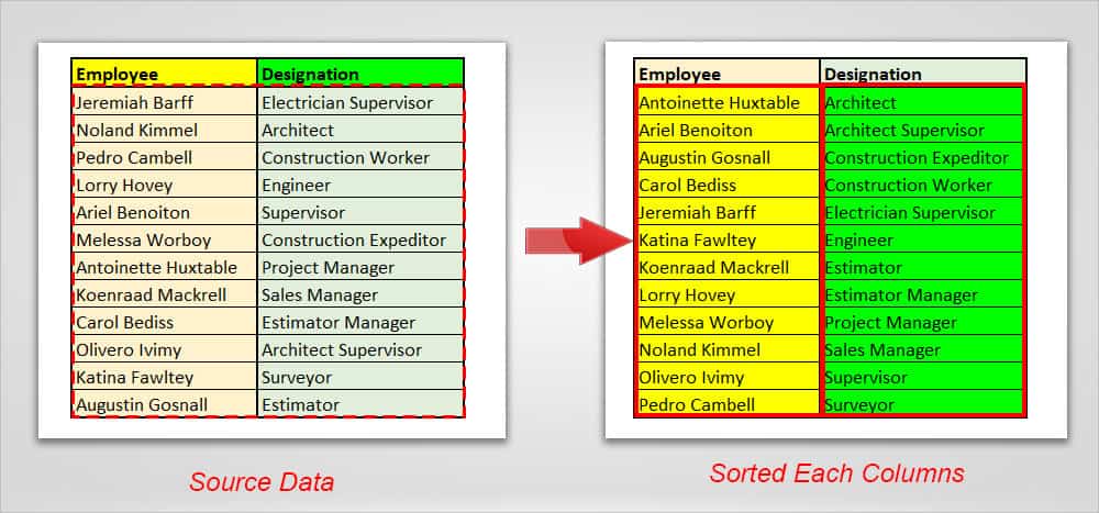
Alphabetize Each Row and Column
Sometimes, you may find the need to sort each row or column individually. To do that, we can use the INDEX, MATCH, COLUMNS, ROW, and COUNTIF functions nested together.
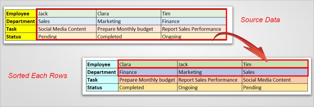
Alphabetize Each Row
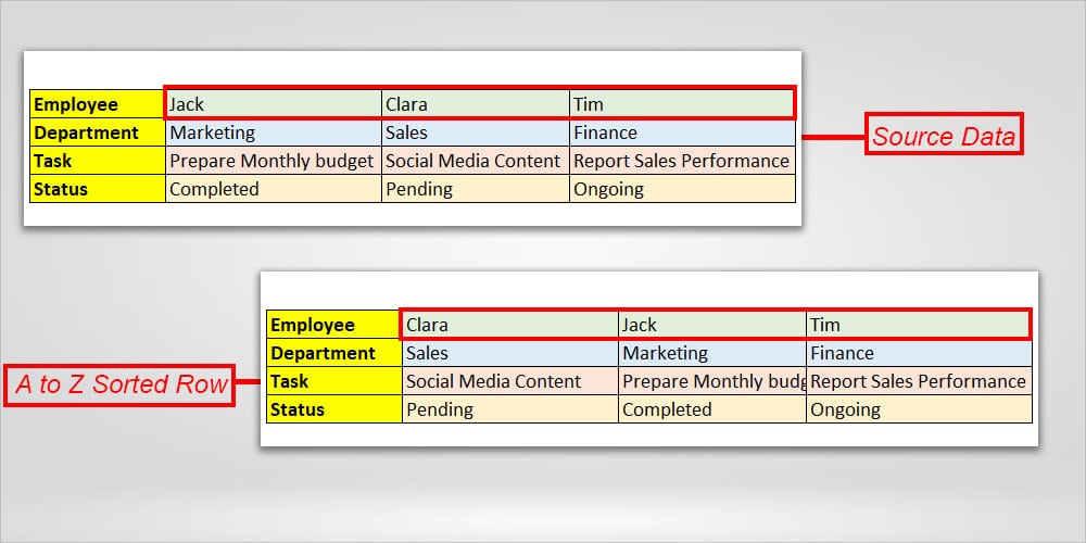
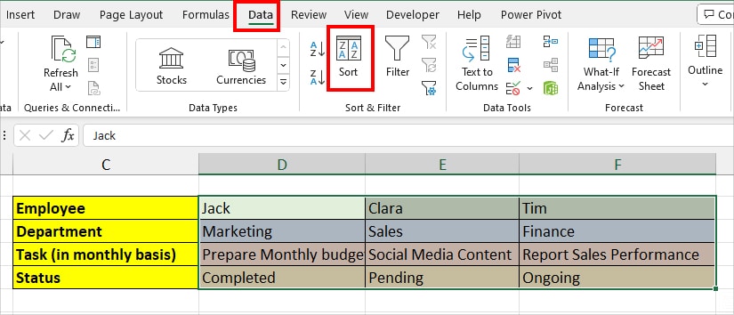
Here, I have a Row of Employee, Department, Task, and Status. I will sort each of the Rows one by one in the A to Z order.
To do that, I entered this formula
=INDEX($C4:$E4, MATCH(COLUMNS($C4:C4), COUNTIF($C4:$E4, "<="&$C4:$E4), 0))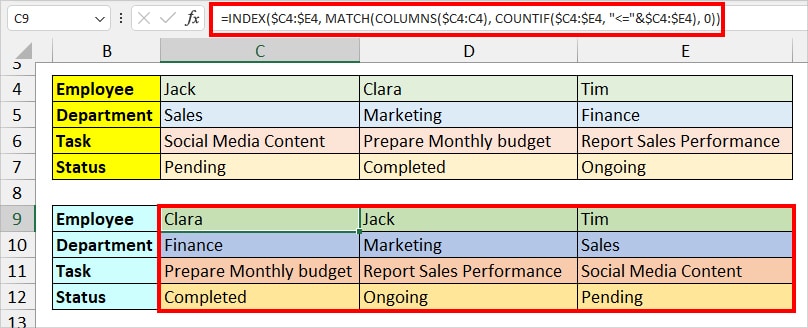
The formula returned the first value from the row. Now, using the Flash-fill, I will copy down the formula to the remaining rows.
To understand the formula, let’s break it down.
COUNTIF($C5:$E5, "<="&$C5:$E5): Returns the total number of non-blank cells.MATCH(COLUMNS($C4:C4), COUNTIF($C4:$E4, "<="&$C4:$E4), 0): MATCH function returns the position of COLUMNS($C4:C4) lookup value from the (2,1,3) lookup array.INDEX($C4:$E4, MATCH(COLUMNS($C4:C4), COUNTIF($C4:$E4, "<="&$C4:$E4), 0)): Finally, the INDEX function returns the value of the position from a Row resulted by MATCH function.
Alphabetize Each Column
In the same way as above, now let us look into the alphabetizing columns one by one in Excel. This time instead of the COLUMNS, we will include the ROW function.
On my Sheet, I have lists of Employees and Designation. Let’s alphabetize both Columns using this formula.
Formula:
=INDEX(C$4:C$15, MATCH(ROWS(C$5:C5), COUNTIF(C$4:C$15, "<="&C$4:C$15), 0))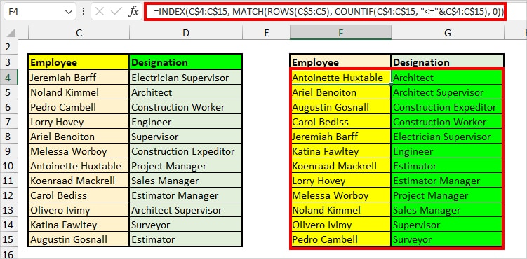
After I got the results, I dragged the Flash-Fill handle to return the rest of the outcomes.