The ROW function in Excel is one of my go-to functions to use when trying to make a function loop through an array. While you can also use the function to simply know what row you’re currently on, it is mostly nested in other functions to re-run them a specified number of times.
Arguments Used in ROW
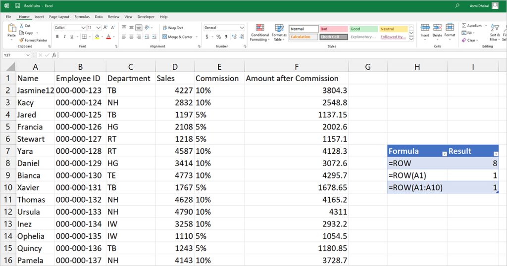
The ROW function is one of the few functions that do not require an argument. When you do not specify an argument, the function will return the row value of the active cell. However, if you specify a cell, the function will return the row position of the specified cell.
Similarly, you can also pass a range in the ROW function. The function will return the row number of the first cell in the range if you press enter. However, if you use Ctrl + Shift + Enter, which is how you enter an array, you will get the row position of the range in individual cells.
The ROW function also works with named ranges, so instead of passing a cell location as an argument, you can also use the name of the range. Take a look at this spreadsheet to learn more about what argument results in what value in Excel.
Applications of the ROW Function
You can use the ROW function to check the position of your active cell. However, the function isn’t as simple as it looks as it is used to create an array, inside or outside a nested formula.
Create an Array
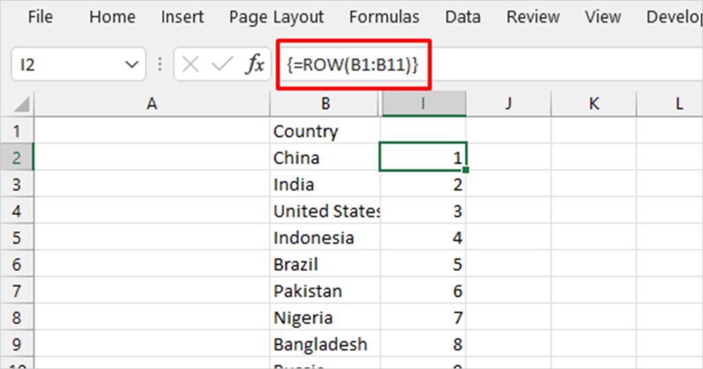
Passing a range as an argument means that you can create an array out of it. For example, if I want to create an array from 1 to 10, my formula would look something like =ROW(B1:B10). What’s really important when you’re trying to create an array is instead of using Enter, you must return your value using Ctrl + Shift + Enter.
Your array should spill vertically in the cells below the cell you enter your formula in. Even if it doesn’t, check the formula bar. If your formula is under curly brackets, then you’ve successfully created an array.
Create a Loop Inside a Formula
As we mentioned before, the ROW function is mostly nested with other functions. Recently, when I covered extracting numbers from a string value, I nested the ROW function with many other functions to create the formula which looked something like, =TEXTJOIN("",TRUE,IFERROR((MID(A2,ROW(INDIRECT("1:"&LEN(A2))),1)*1),""))
Let, A2 = 123abc
Let’s not go into detail about the entire formula and focus on the role of the ROW function. Inside the formula, the ROW(INDIRECT(“1:”&LEN(A2))) returns an array, which is the length of the cell A2. In our example, we’ve taken cell A2 to be 123abc so our array will be {1,2,3,4,5,6}.
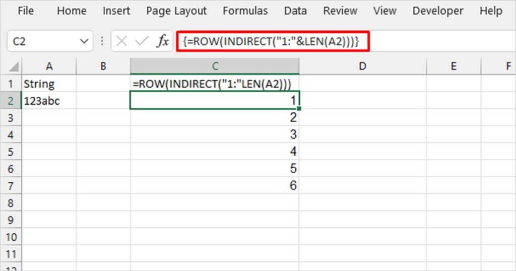
The MID function will then loop six times to return the value for each position of cell A2. This is how the ROW function can create a loop inside a formula, how useful!
Use ROW() in Conditional Formatting
You can use the ROW() function to highlight every other row in conditional formatting! As the ROW() function returns the position of every row, you can write a formula to format every cell that the ROW() function returns an even number for.
We will be nesting the ROW() function inside MOD() for this. The MOD function is used to get the remainder when dividing a number. When you divide an even number by 2, the remainder is always 0. Similarly, when you divide an odd number by 2, the remainder is always 1. We will be using this logic to construct our formula.
- Open your worksheet and select the range you wish to apply conditional formatting.
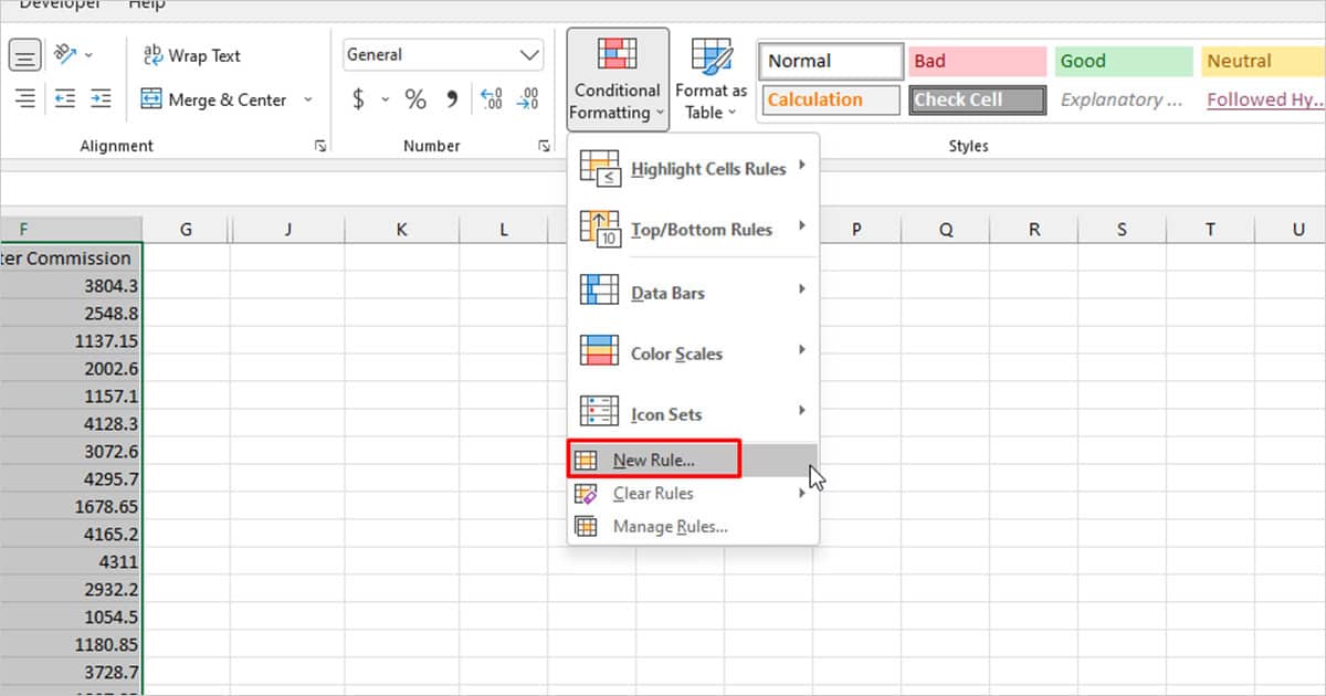
- On the Home tab, select Conditional Formatting.
- Choose New rule from the fly-out menu.
- Under Select a rule type, select Use a formula to determine which cells to format.
- Depending on what cells you wish to format, enter one of these formulas under the Format values where this formula is true:
- To highlight every even cell, use the following formula:
=MOD(ROW(),2)=0
- To highlight every odd cell, use this formula:
=MOD(ROW(),2)=1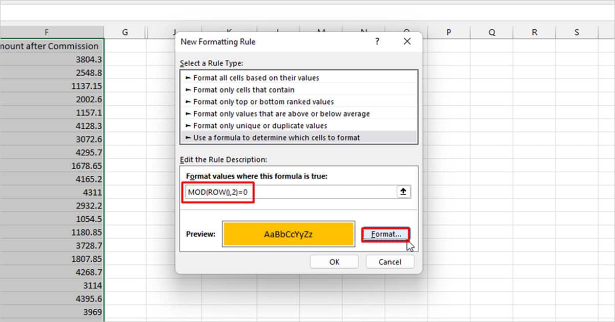
- Click the Format button to set a format.
- To confirm the changes, select OK.
You can also highlight different rows using the ROW() function in conditional formatting. For instance, you can format every fourth row using the MOD(ROW(),4)=0. Similarly, you can nest other functions with the ROW() function to create your own logic to highlight rows in Excel.
What is the “You’ve entered too many arguments for this function” Error While in the ROW() Function?
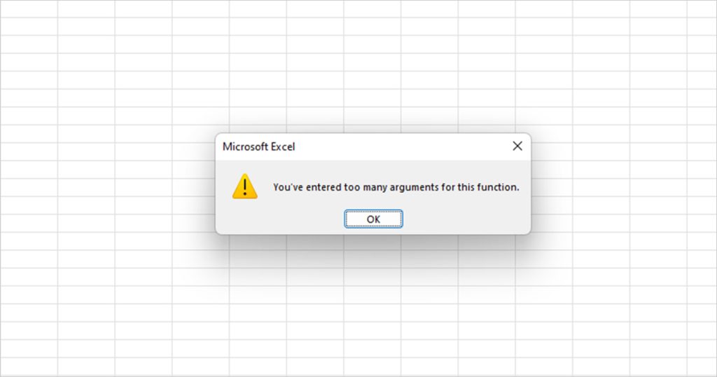
Now that we know that you can create an array using the ROW() function. Using this theory, you passed cells A1, A2, and A3 as arguments in the ROW() function. Wait, instead of getting an array of 1,2,3 in the corresponding cells, you received the “You’ve entered too many arguments for this function”. Is this a glitch?
Actually, it isn’t a glitch. The ROW() function actually doesn’t take more than one argument. If you want to create an array, instead of referring to individual cells, pass a cell range as the argument.
So rather than passing A1, A2, and A3 as arguments, if we pass the range A1:A3, voila! There’s our array.
ROW() Function not Creating an Array?
When I first started dealing with arrays, I almost always fail in creating one using functions. If the ROW() function isn’t creating an array, as in if it’s only returning one value, it’s because you used Enter instead of Ctrl + Shift + Enter to return the value.
To check if your formula has been registered as an array, select the cell will the formula and check the formula bar. Your formula must be inside curly brackets if it’s been passed as an array. If not, select F2 to edit the cell and use Ctrl + Shift + Enter to pass it as an array.