How to Make and Use Pivot Table in Excel (Beginners Guide)

Excel’s Pivot Table can be both mind-blowing and intimidating for beginners who are trying to use it for the first time.

Although PivotTables are best for summarizing huge data, it can go wrong when you don’t know how to place the rows/columns in the right fields. 

So, today, I will be guiding you through the step-by-step guide on how to make and use PivotTable the best way in Excel.

What is a Pivot Table?

In Excel, we all have a Master Spreadsheet that contains raw data with large rows and columns. From that source, we often need to calculate the sum, and find out the highest sales of an item based on the total, or an average of values.

While you could use the SUM or other functions, it can get pretty messy in a massive sheet.

So, that’s where the Pivot Table comes in as the Knight in Shining Armor. Using the Pivot Table, you can effortlessly prepare an insightful summary report of your data like cross-tabulation.

It’s also one of the pro tips to increase your productivity and save time. 

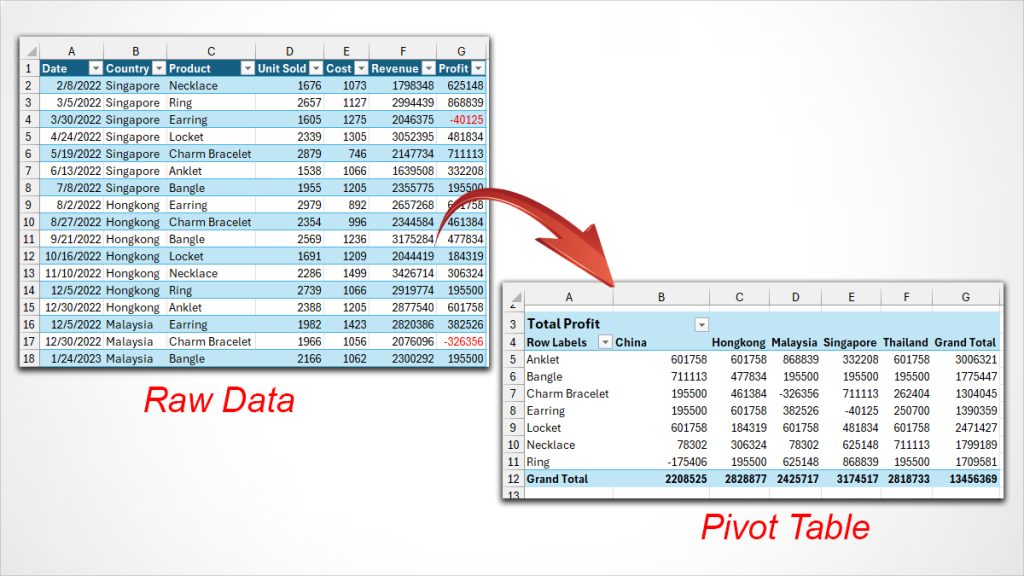
The best part is that the data is organized in such a way that even a beginner can read and analyze the information without any difficulty. 

How to Add a Pivot Table?

Step 1: Prepare Data Source

Usually, it is most likely that your original raw data might not be in the best format. By that, I mean sheets with blank cells, no column headers, errors, and so on. 

So, before you insert a Pivot Table, let’s do a little touch-up to clean and organize your data.

Here are some of the tips.

• Firstly, check if there are Blank cells in your Sheet. In case your data has blank cells, delete them immediately.
• Column Headers are very important to construct the Pivot Table. So, insert titles for your columns.
• To make your Pivot Table more dynamic, change your data into Table Format. Select all and enter the Ctrl + T keyboard shortcut. On the Create Table, click OK. This ensures that the Pivot Table immediately includes the extra rows and columns you add.
• Once you apply Table Format, rename the Table. For that, click on the Cell and go to the Table Design. In the Properties group, type a New name.
• Delete Total or Subtotal Rows from your data. Since we are about to create a subtotal using the Pivot Table, such rows would be redundant.

Step 2: Add Pivot Table

If your data is ready, now let’s create a Pivot Table. 

Firstly, select Table range and head to the Insert Tab.

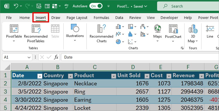
In the Tables group, select PivotTable. Then, pick your source:

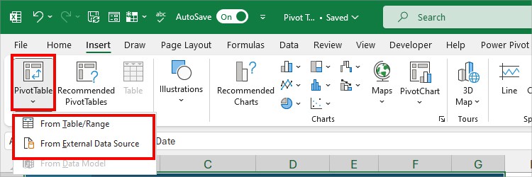
1. From Table/Range: Choose this to insert a Pivot Table for your existing data. Then, fill in the given information.
   
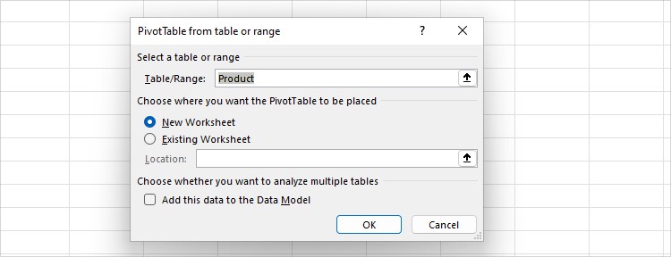
   • Table/Range: Type Table Name.
   • Location: Choose between New Worksheet or Existing Worksheet to load your Pivot Table. If you select Existing, enter the Ranges to import too. Hit OK.
   • Add this data to the Data Model: Tick this option to insert your current Table/Range to data mode.
2. From External Data Source: Select this if your data is not in the current sheet.
   
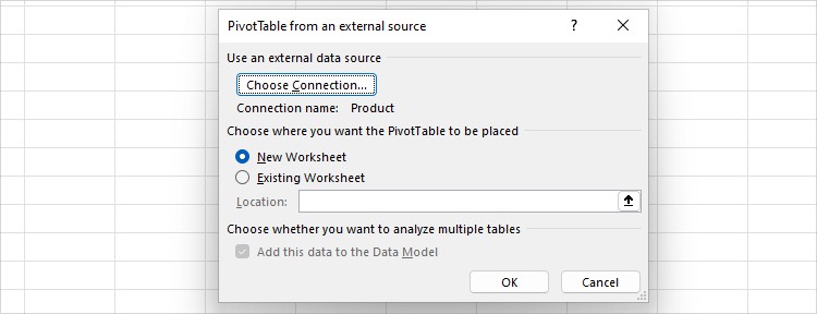
   • Choose Connection: Click this Button to select the external Table/Range. After that, choose data from Connections or Tables. In case the workbook is on a PC, click Browse for More and import the workbook. Finally, hit Open.
   • Location: Pick a New Worksheet or Existing Worksheet to load the Pivot Table. For the current sheet, enter the Cell References as well. 

After you have entered all the details, hit OK. 

Step 3: Edit Pivot Table Field

At first, you will only see an empty Pivot Table Field. To create a summary, you must select the Fields. 

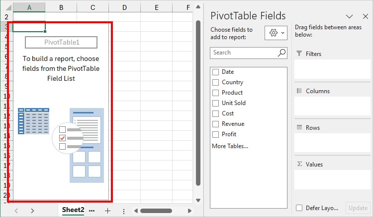
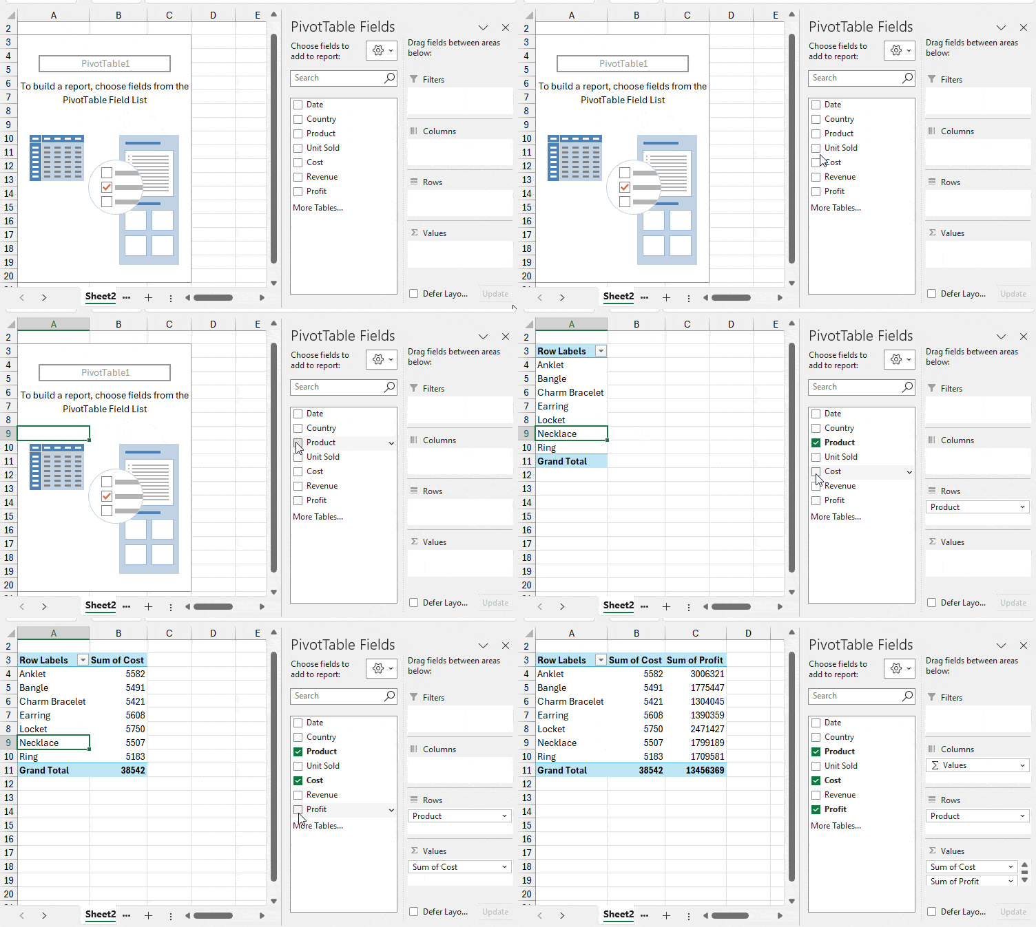
Hover over the PivotTable Fields. Then, tick the boxes for Column Headers to display as per your need.

Let us consider that I have the Date, Country, Product, Unit Sold, Cost, Revenue, Profit, and Target Sales Fields.

As soon as I checkmark the boxes for Product, Cost, and Profit, I will have a Grand Total in the Pivot Table.

Step 4: Adjust Row and Column Fields

Sometimes, the Rows and Columns in the Pivot Table aren’t in the proper Field. 

For example, I want to show the units sold of each Product for different countries. But, I have both Product and Country in the Row Field which makes my Pivot Table look huge and hard to read.

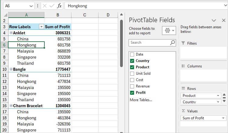
To address that I will drag the Country column to the Columns section in the PivotTable Fields panel. 

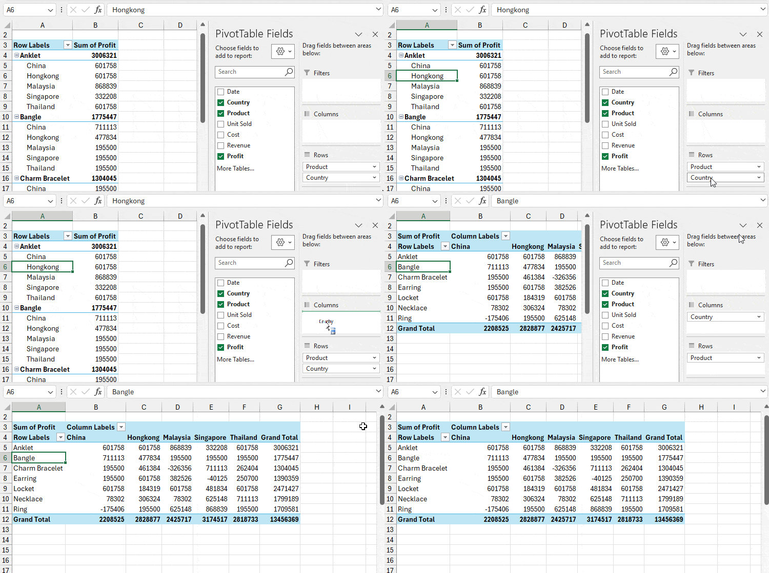
Just like that, you could drag the Fields from Column to Row and vice versa as required. 

How to Use a Pivot Table?

Inserting a Pivot Table is easy. However, most people often struggle with its usage part. 

So, now, I will explain each feature and menu in detail to help you use Pivot Table at its utmost potential. 

Change Number Format

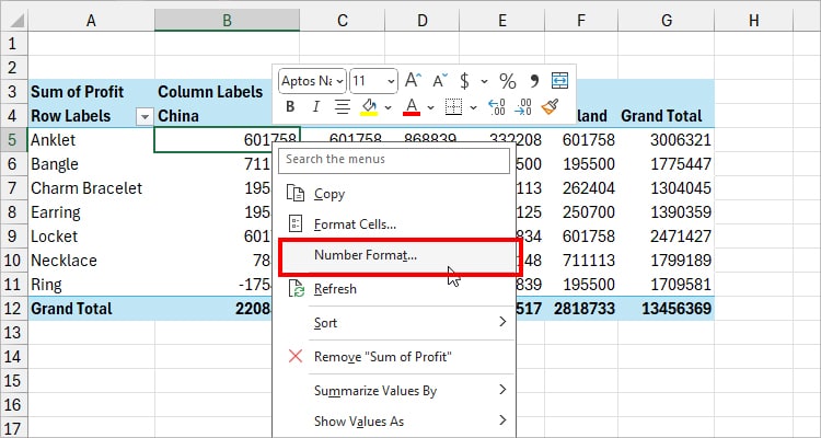
If you need to change the Number Format, you could do it in your Pivot Table itself. For that, right-click on the cell and pick Number Format in the context menu. 

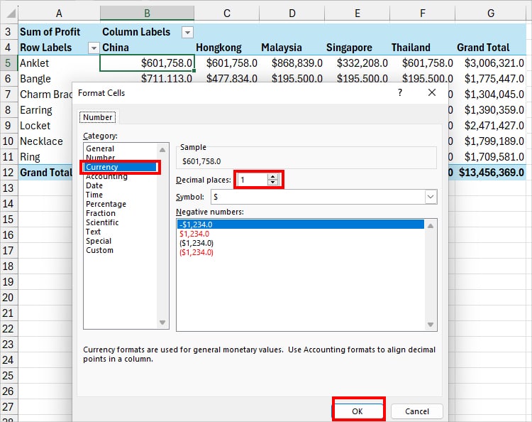
On the Format Cells window, select the Category, choose a Format, and hit OK. For Instance, here, I chose to apply the Currency format with 1 decimal place. 

Show Value As

Next, this is one of my favorite features of the Pivot Table. Using the Show Value As menu, you could display calculated fields in separate ways without having to compute them manually.

Let’s say, here, I have the total profit for each product in numbers. But, I can show them as % of grand total without even calculating it.

Isn’t that smart and easy?

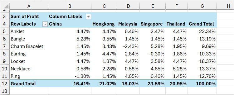
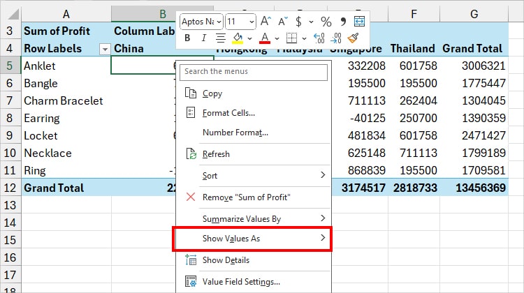
To do that, right-click on one of the cells in your Pivot Table. Then, click Show Values As.

Choose your option.

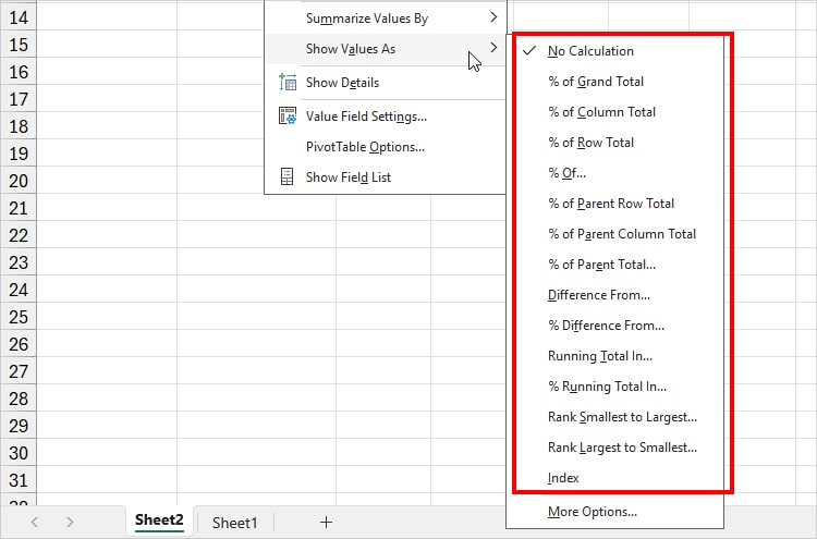
Also, before you select, you can hover over each option to see what the menu will display. Or, check from the Microsoft Excel’s Official Site. 

Summarize Value By

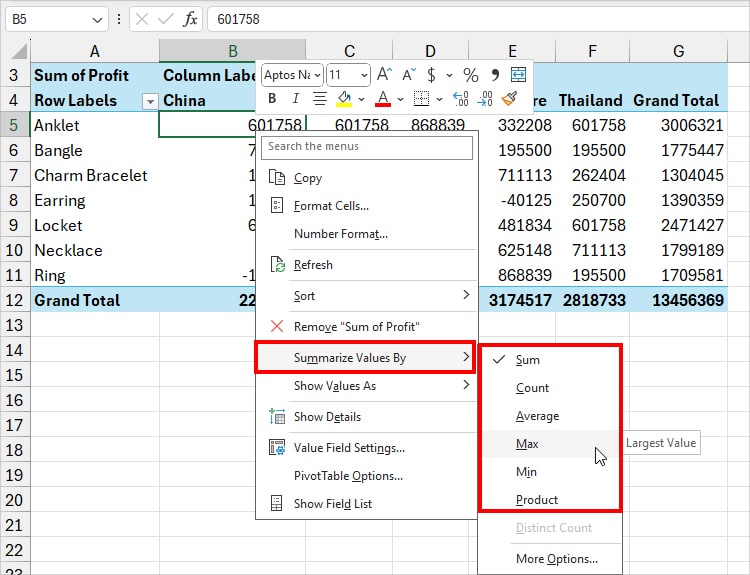
Pivot Table’s calculation is not only limited to the Sum. You could summarize your data by Minimum Value, Product, etc. 

For instance, your Grand Total shows the Sum of values by default. But, instead, you can show the Maximum numbers in the Grand Total row.

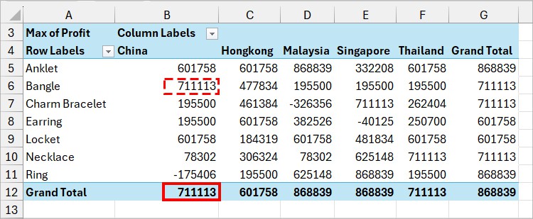
Right-click on the Number. Choose Summarize Values by and select options from Count, Average, Min, Max, Product, etc.

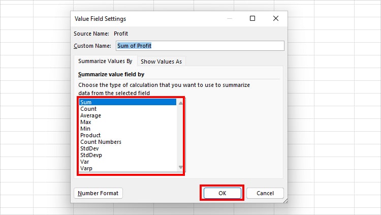
Or, to explore more, select More Options. Then, on Value Field Settings, scroll and pick a Calculation type. Click OK.

Remove Grand Totals and Sub Totals

By now you must have understood that the Pivot Table calculates the Grand Total and Sub Total by default for all items. 

But, let’s assume, you just want to have the sum in the Pivot Table. Now, this is a little tricky part as you cannot select and hit the Delete key to remove Grand Total.  

Instead, you need to click a cell in the Pivot Table and head to the Design Tab. 

Expand the Grand Totals menu and choose one of the options.

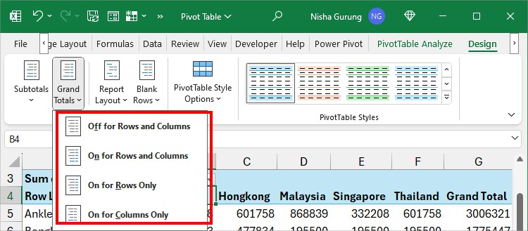
• Off for Rows and Columns: Delete the Grand Total from both Rows and Columns.
• On for Rows Only: Keeps the Grand Total for Rows and removes for Columns.
• On for Columns Only: Eliminates the Grand Total for Rows and shows for Columns only. 

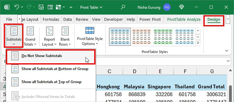
Similarly, to remove Subtotals, click on Subtotals > Do Not Show Subtotals. 

Update Table Layout and Design

If you do not like the current look of your Pivot Table, you can change the Layout as you wish. There are various layout options to organize your Pivot Table. 

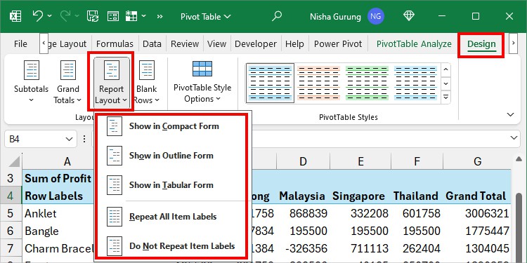
In the Design Tab, click Report Layout and choose one.

Here’s how each Layout would appear. 

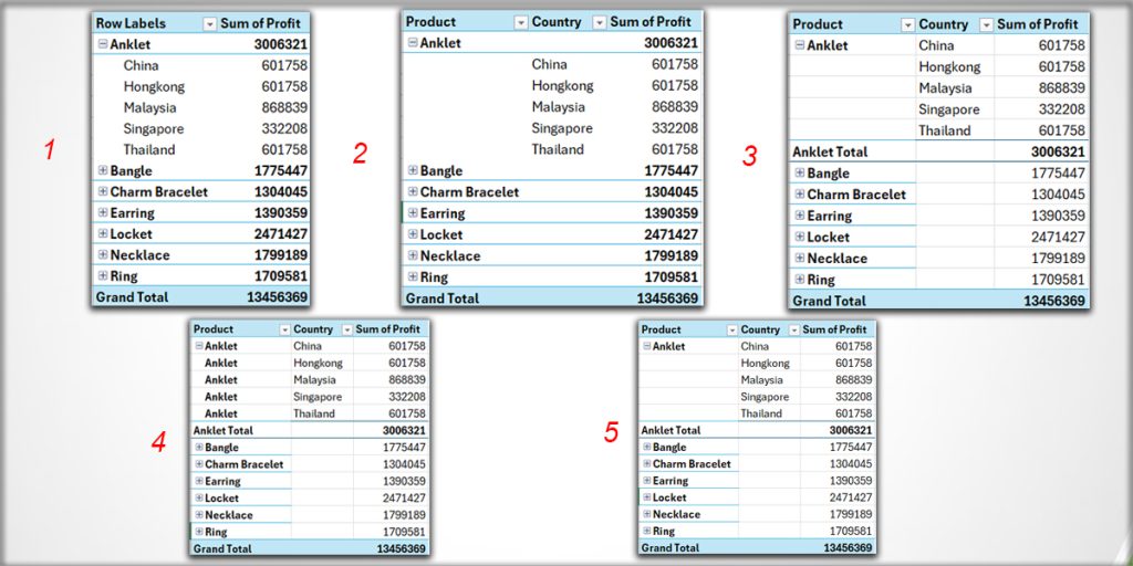
• Show in Compact Form
• Show in Outline Form
• Show in Tabular Form
• Repeat All Items Labels
• Do Not Repeat Item Labels

Sort in Pivot Table

You could sort your data alphabetically or in ascending/descending order to make your data analysis easier. 

For Example, if I reorder my values from highest to lowest, I can quickly know the most sold product based on the sum.

To rearrange, right-click on the Cell > Sort. Then, pick any one option.

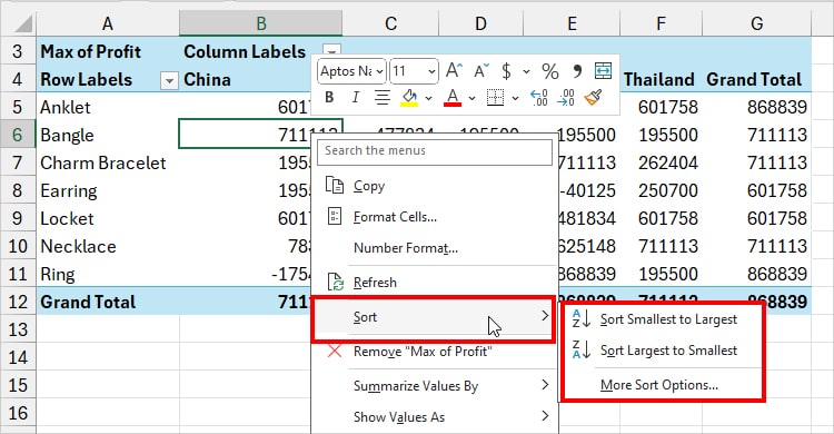
• Sort Smallest to Largest: Ascending or A to Z order.
• Sort Largest to Smallest: Descending or Z to A order. 
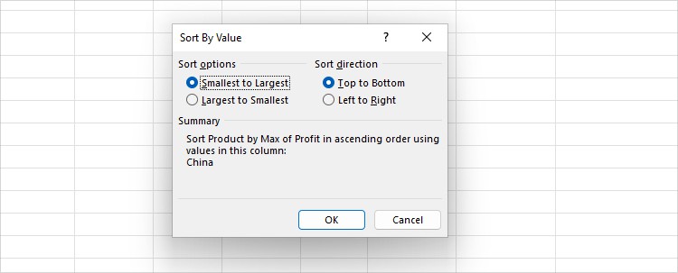
• More Sort Options: Specify both Sort options and Sort Direction (Top to Bottom or Left to Right). Click OK.
  

Filter Data

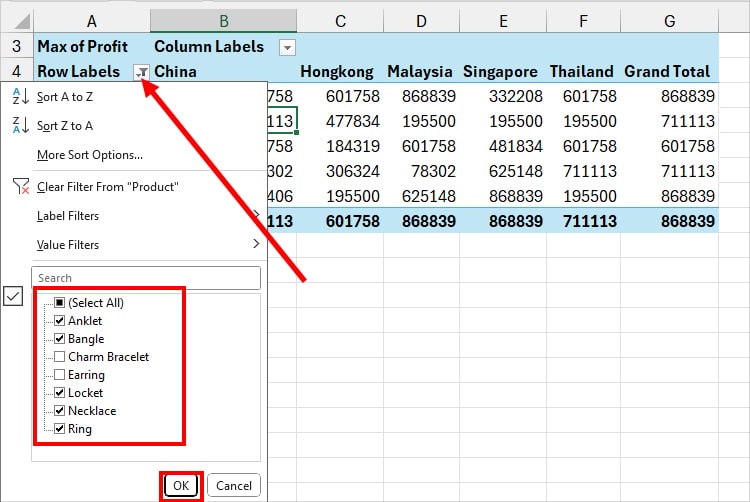
Pivot Table already has the Filter button. Additionally, if you look into the Field Settings, you’ll also find a separate Filters section like the Column and Row. So, filtering out values is simple. 

Click the Filter button and Untick the boxes for the information you want to hide. Once you’re done, hit OK.  

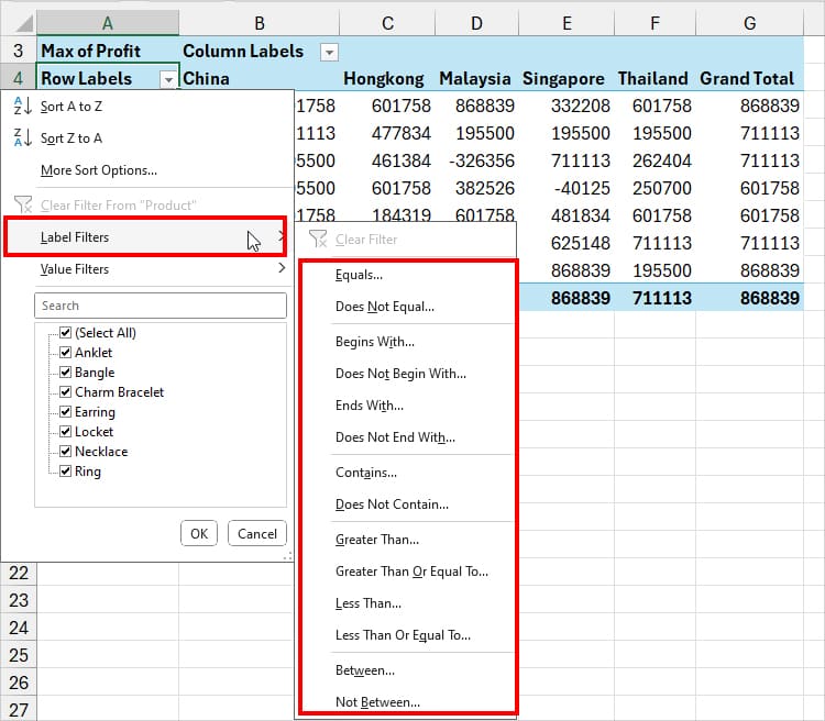
But, if you wish to filter values with specific criteria, expand the Filter button >  Label Filters > Condition. Then, enter the Header and click OK. 

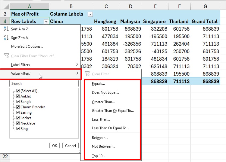
Just like that, to do a conditional filter for values, click Filter. Select Value Filters > Criteria. On the prompt box, enter the Value and hit OK.

Add Slicers 

Do you know that the Pivot Table has an amazing feature named “Slicer” to filter data?

It is the most interactive way of filtering out values. Honestly, it is my go-to filter tool whenever I need to present my data in a more visually appealing and fun way. 

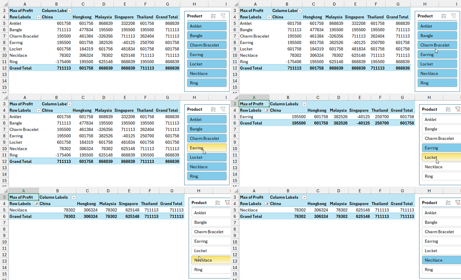
The interesting part is Slicers works with Pivot Charts too which is a win-win situation here. You could filter the information in tables as well as charts at the same time. 

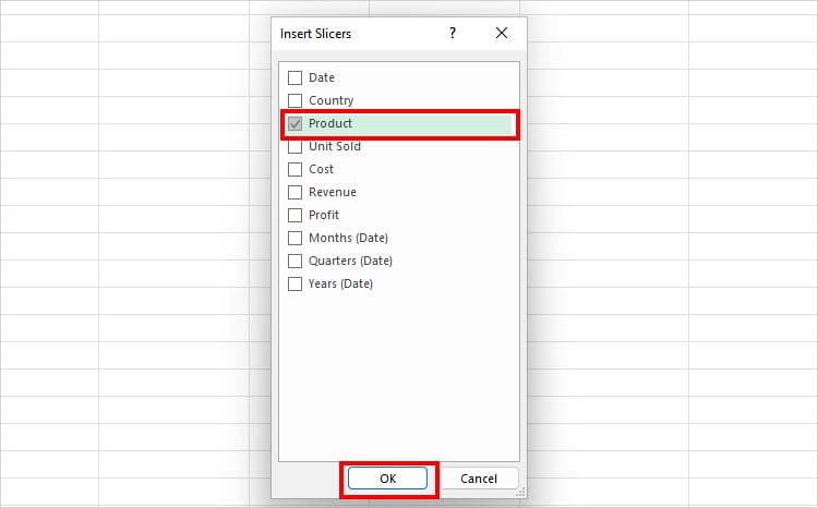
To insert, go to the PivotTable Analyze Tab and click Insert Slicer.

Choose a Category and hit OK.

If you want to deep-dive into this feature, we have an entire article on How to Use Slicers in Excel. 

Insert Pivot Chart

Sometimes, you may need to graphically represent your Pivot Table information. In that case, construct a Pivot Chart to make your data analysis more insightful. You could add all kinds of charts such as Column, Line, Pie, Area, Stock, and many more. 

But, are the Pivot Charts different from standard Excel Charts?

Well, although the charts appear the same as standard ones, there’s a major difference in the Source. While the Excel chart is linked to sheet data, Pivot Charts are connected to PivotTable. 

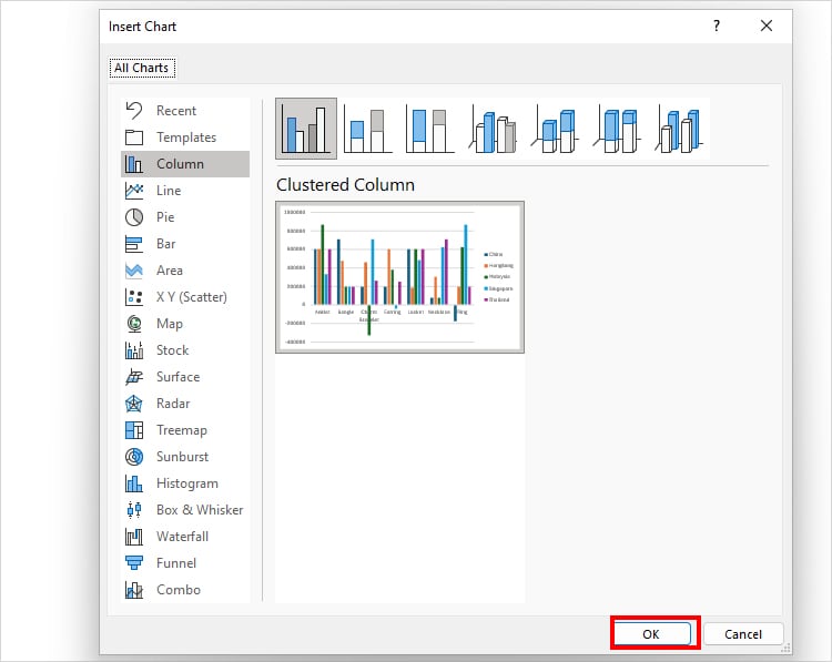
To insert, go to the PivotTable Analyze tab and select PivotChart. 

On Insert Chart dialogue, select Chart and click OK. 

Group Data in Pivot Table

For a more detailed categorization of items in your Pivot Table, you could use the Group feature.

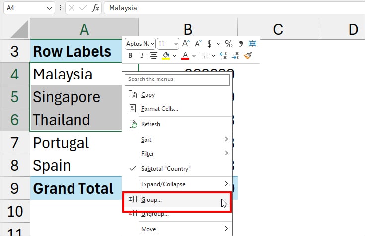
For example, if your table has lists of countries, you can them based on regions like Europe, Asia, etc.

Select the labels you want to keep in one category. Right-click on the selected items and click Group. 

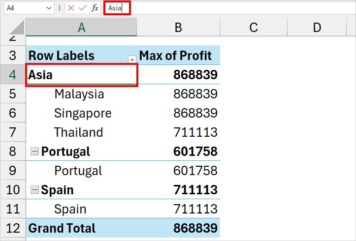
By default, the name will be Gorup1, Group2, etc. To rename, click on the Group header cell. Then, type a new title in the (fx) formula bar.

In case your Formula bar is not showing, here’re ways to fix it.

Refresh Pivot Tables

Updated new information in your source data? 

Don’t worry! You don’t have to create new Pivot Tables every time as there’s a Refresh option.

Click the PivotTable Analyze Tab. From the Data group, select Refresh. It’s also helpful for your Pivot Charts. 

Move PivotTable

There can be instances when you need to transfer your Pivot Table to another location. During such a situation, shift your data without affecting other work in your sheet with these two steps.

From the PivotTable Analyze tab, click on Move PivotTable.

On Move PivotTable, select a Location and click OK.

• New Worksheet: Excel creates a blank sheet and loads the Pivot Table.
• Existing Worksheet: Move the table in the same sheet but in a different area. In the Location field, specify your cell range. 

Delete Pivot Table or Unpivot

If you no longer want to use Pivot Table, select All. Right-click on your selection and click Delete.

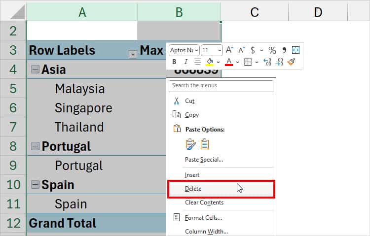
To know the other 6 ways to get rid of a table, check out the “How to Delete a Pivot Table in Excel” article guide. 

Or, in case you want to revert your PivotTable to its original state without deleting it, there are 4 simple steps to do so. We’ve covered it in “How to Unpivot Data on Excel.”

Can You Create a Multiple Pivot Table?

Above, we just created one Pivot Table. But, you can add as many Pivot Tables as you want. This is especially helpful when you need to analyze the information based on different criteria.

For Instance, here, from the same data source, I made these Pivot Tables to create a Dashboard in Excel.

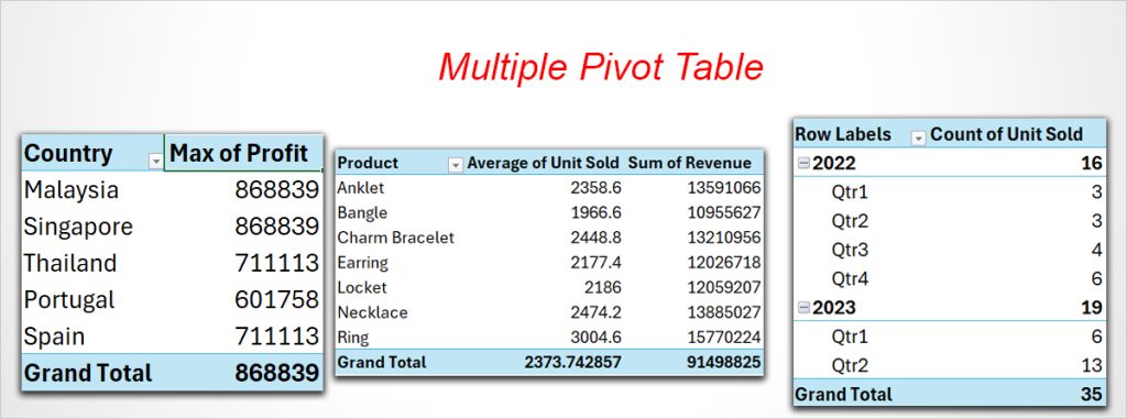
It’s up to you if you want to repeat the above Steps 2 and 3 to add. All you need to do is filter out and select only the Column headers you want to analyze. 

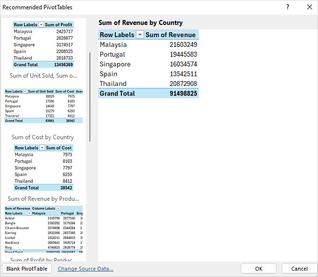
Besides, another way to construct is by using the Recommended PivotTables feature. From Insert, click on Recommended PivotTables. 

In the Window, choose a Pivot Table and click OK.