For a large set of rows in Excel, adding a Number list can help you easily pinpoint the exact position of a row. But, since Excel lacks in default Number list menu, most beginners might input the sequential values one by one in the cell range. If you are also doing this, you aren’t going anywhere with this speed!
In fact, Excel has even more smart ways to number rows. You could use tools like Auto-Fill and Series to automatically add the numbers. These tools literally do all the work for you. Besides, if you want to skip blanks and apply filters, you can always use the Functions.
Static Numbering VS Dynamic Numbering
Below, I have mentioned different method that does Static and Dynamic row numbering in Excel. Before you start, identify which type of numbering is appropriate for your dataset.
Static Numbering stays intact even when you add or delete a row. It’s useful only if you want to have numbered lists for your rows.
On the contrary, Dynamic Numbering auto-updates the values regardless of the changes you make in the row. For example, if you add a new row, you’ll immediately have a number.
Use Auto-Fill and Fill Series for Static Numbering. For Dynamic Numbering, you can opt for ROW, SUBTOTAL, or IF, ISBLANK, and COUNTA functions.
Use Auto-Fill Feature
Excel has this fantastic “AutoFill” feature that automatically fills the values when there’s a similar pattern in the cell ranges. When you enter a number sequentially in a cell, the tool identifies that pattern and auto-numbers all the rows. This is my go-to method on a daily basis.
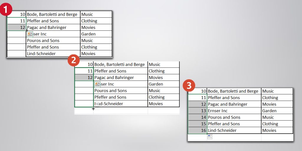
Firstly, enter 1 in the first cell. Then, in the second cell enter 2. Now, select both cells. Hover over the bottom right corner of the selected cells. Once you see the Plus cursor, drag it down and drop to autofill the number for the remaining cells.
In case, you still want to add more numbers, you don’t have to reselect the entire cells from the first. Just select the second last and last number. Then, extend the Auto-Fill Handle all the way down.
Use Fill Series
Although the Auto-Fill feature is very easy to use, you might lose control when you have to drag the fill handle all the way down. So, it isn’t much convenient to number rows of bigger spreadsheets. In that case, we’ve another method where we will be using the Fill Series menu.
From the Fill Series, you can actually determine the custom Start and End Value. Therefore, you will get the exact numbering which saves you from re-adding or deleting values.
- Firstly, type in number 1 in the first cell.
- In the Home Tab, navigate to the Editing section. Click on Fill > Series.
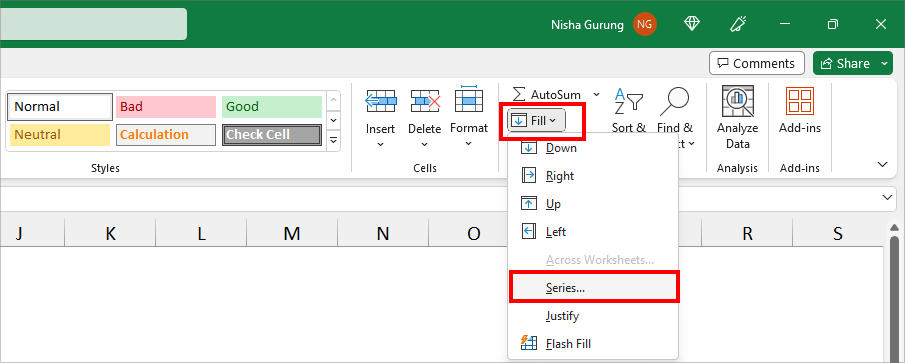
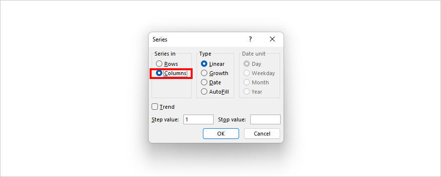
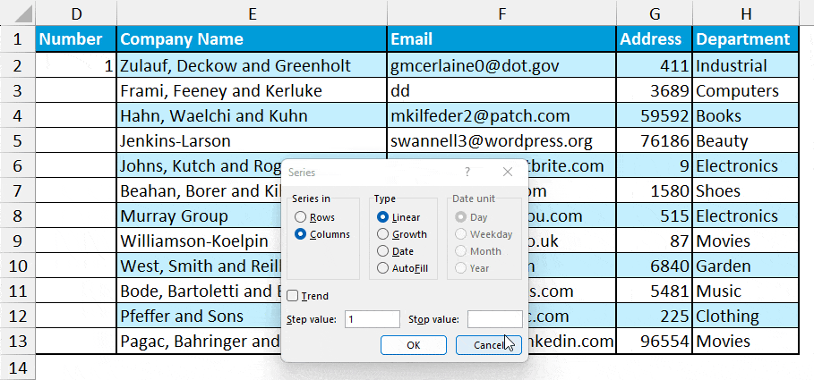
- On the Series dialogue box, choose Columns for Series in.
- On Stop Value, enter the Last Number and hit OK. You’ll have numbers in cells.
Use ROW Function
Auto-Fill and Fill Series are both effective as long as you do not have to insert or delete rows. But, if you want the numbers to be dynamic, you can use the ROW function.
In Excel, the ROW function is used to reference the row number of cell or cell ranges in the spreadsheet. So, this function doesn’t really have the function arguments. The reference in the Function argument is absolutely optional.
Syntax: =ROW([reference])If you leave the argument of the ROW function empty, it returns the position of the active cell. So, we can use that reference to subtract the row by a value and return a number. Remember, here, the active cell plays a huge role.
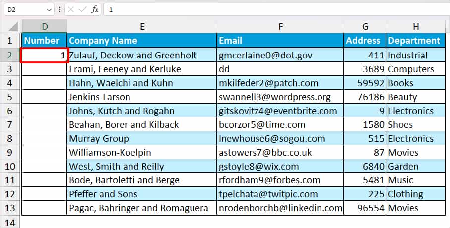
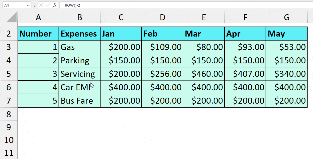
Example: Suppose, cell D8 is my first cell that contains information in the sheet. I want to start numbering from there onwards. To do so, I entered the given formula.
=ROW()-7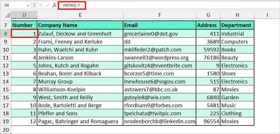
I got 1 in cell D8. Then, I used the Auto-Fill handle to number the rest of the cells. The logic is pretty simple. Just subtract the current row number by a value that would result in 1. In my case, 8-7 = 1.
To give another example, if my active cell was B3, the formula would be =ROW()-2.
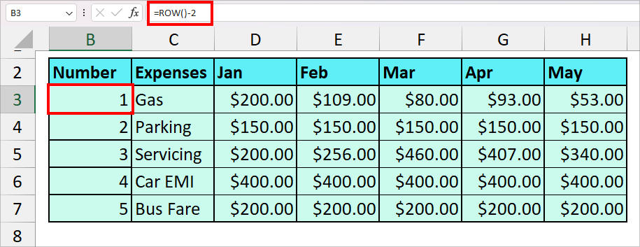
Now, if I delete a row, the values will update accordingly.
Use the ROW Function in Table
When you do numbering for a normal cell range, you would have to use other tools like Flash-Fill to input values for a new cell. But, if you have a table, it automatically fills the number until the last cell.
This method is for users who already have a table range. Even if you don’t have you could create a table by pressing the Ctrl + T and confirming on the prompt box.
On the first cell of the Number Column, enter this formula
=ROW(Table6[#All])-0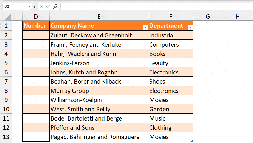
Keep in mind, as I have mentioned above, that the value you subtract depends on the active cell of numbers. To get 1 on cell D2, I subtracted by 0.
Also, when you add extra rows to the table, the numbered lists will also be included.
Use IF, ISBLANK, and COUNTA Function
While the ROW function is helpful in automatically having the number for new rows, it could be an issue if you’ve left the cells blank intentionally. To address this, we will nest the IF, ISBLANK, and COUNTA functions together to skip numbering for blanks.
=IF(ISBLANK(C2), "", COUNTA($C$2:C2))After I entered the formula, I dragged down the Flash-Fill handle for other cells. As you can see from the image, the formula skipped numbering in the blank cells and re-continued from the cell that has value. So, how exactly did the formula do this? Let’s find it out below.
- COUNTA($C$2:C2): Firstly, the COUNTA function counts and returns the number of non-empty cells. In our case, we had a value in cell C2 so it resulted in 1.
- ISBLANK(C2): The ISBLANK function returns TRUE if cell C2 is empty and FALSE when there’s a value. We got FALSE in this instance.
- IF(ISBLANK(C2), “”, COUNTA($C$2:C2)): Finally, the IF function tests ISBLANK(C2) logic and returns “” when the value is True and 1 when the value is false.
Use SUBTOTAL Function
There can be instances when you need to delete, move, or copy-paste the filtered rows. After filtering the rows, you may have noted that the numbers stay as it is even for the hidden items. As a result, you’ll have messed up the numbering.
If you need to apply a filter, I recommend you use the SUBTOTAL function to add the numbers for rows. Using this function, the number becomes dynamic for filtered rows.
Firstly, if you have the Filter tool on, enter Ctrl + Shift + L keyboard shortcut to turn it off. Then, in the Number column, enter the given formula.
=SUBTOTAL(3, $C$2:C2)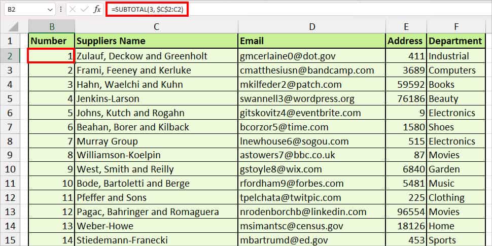
After you get the result, use the Auto-Fill. By, entering the 3 in the formula, we’re specifying the SUBTOTAL to use the COUNTA function. So, it checks whether the $C$2:C2 contains a value or not. Then, returns a value. Here, we got 1.
Now, again, press the keyboard shortcut to enable the Filter. This time when you filter the rows, the numbering changes automatically.