If you have downloaded Excel spreadsheets from an external source, it might not be in the best condition as you expected. It could contain a lot of spilled data, inconsistent formatting, formula errors, duplicates, too many highlights, and so on. You wouldn’t want to use such a messy worksheet, especially for professional purposes. To maintain the standard, you can clean your Excel data.
I know you may feel overwhelmed when you do not know where to begin from. But, I have compiled 13 methods that’ll help you to clean your data. Additionally, at the end of this article, you can also learn pro tips to maintain your spreadsheet nice and organized.
Fit Text
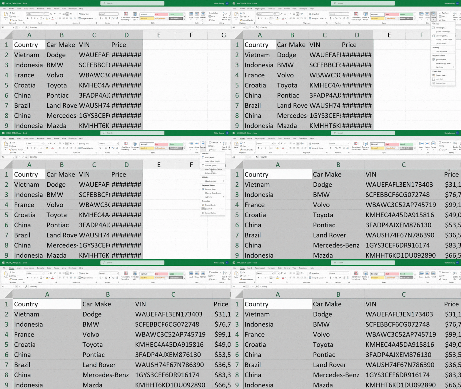
In order to have a clean spreadsheet, your texts and paragraphs should fit the cells. Your spreadsheet will definitely look cluttered if you have data spilling all over the columns. You might as well encounter the ##### error when the text is too large. To fit texts, you can adjust the Column size or use the Wrap Text menu.
If you have smaller text, select the cells and resize the column width using the given keyboard shortcut. As it’s a ribbon shortcut, press each keys one by one.
Shortcut Key: Alt, H, O IAlternatively, you can also change the column size from Excel’s Home Tab.
- On your worksheet, select the Cell ranges.
- From Home Tab, click on Format > AutoFit Column Width.
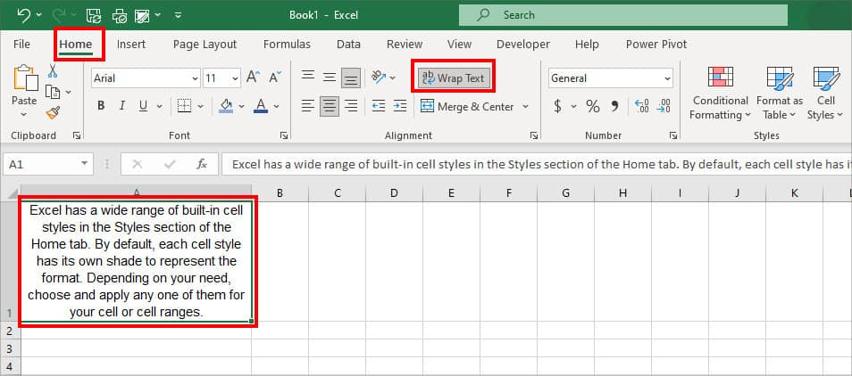
For longer paragraphs, stretching the column size won’t be most effective as it affects your entire column. In that case, you can use the Wrap Text menu. Select the Texts and go to the Home Tab. From the Alignment group, click on Wrap Text.
Clear Format
While formatting your Excel spreadsheet can help increase data readability, it can look messy if you’ve gone overboard with it. For example, exaggerated highlights, inconsistent cell styles, unnecessary hyperlinks, line breaks, and so on. To keep it clean, you can Clear all Formats at once using this keyboard shortcut.
Keyboard Shortcut: Alt, H, E, FIf you’re not into shortcuts, you can always opt for the Excel Ribbon menu.
- Select the entire data using Ctrl + A keyboard shortcut.
- On Home Tab, click Clear > Clear Formats.
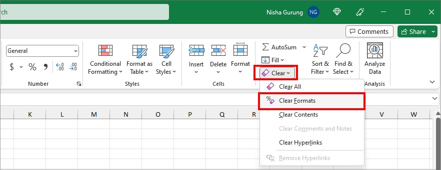
Now, once you’ve removed the formats, you can apply highlights, cell styles, and themes as per your preference. But, make sure to keep it simple and consistent to have a professional spreadsheet.
Change Text Case
When you import external data into your spreadsheet, chances are the texts might be in both lowercase and uppercase mixed. Such inconsistent text cases not only can be hard to read but also impact the calculations. This is because some of the Excel functions are case-sensitive.
So, it’s better to convert the text case using the UPPER, LOWER, PROPER function.
Here, we have provided an example of converting your text to all three uppercase, lowercase, and first-letter capital. Take a reference of the formula and use any one as per required.

| Text Case | Function | Word | Formula | Description |
| Lowercase | LOWER function | Product Management | =LOWER(“Product Management”) | The LOWER function returns all the text strings in small letters. It returned product management as an output. |
| Uppercase | UPPER function | business development | =UPPER(“business development”) | The UPPER function returns the entire text string in capital letters. As a result, we got BUSINESS DEVELOPMENT. |
| First letter capital | PROPER function | sales manager | =PROPER(“sales manager”) | The PROPER function returns all the initial letters of a text as capital letters and converts the rest into lowercase. So, the formula returned to the Sales Manager. |
Trim Space
As spaces are barely noticeable, it’s most likely your texts may contain a lot of unnecessary spaces in them. Many users might not consider spaces as much of an important factor in Excel. But, it actually affects the formula usage which is why you need to remove spaces.
Although there is no default menu to remove spaces, Excel has the TRIM function built for this purpose. The TRIM function deletes all the irregular spaces from the specified text string and keeps only the single ones. Here’s how you use the TRIM function.
Example: Suppose, you want to delete spaces from the text “ College Station.” For this, your formula would be
=TRIM(" College Station")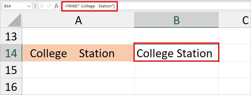
The formula returned College Station as an output.
Remove Duplicates
Do you have duplicates in your data? Sometimes, the duplicate values are just unnecessary in your Excel spreadsheet which only increases the data size. It’s better you remove the duplicates to make your spreadsheet nice and clean. Again, to do this quickly, we have a keyboard shortcut.
Shortcut key: Alt, A, MThere’s also a default Remove Duplicates menu in Excel ribbon if you don’t prefer shortcuts.
- On your sheet, enter Ctrl + A to select data.
- Go to Data tab. On Data Tools, click Remove Duplicates.

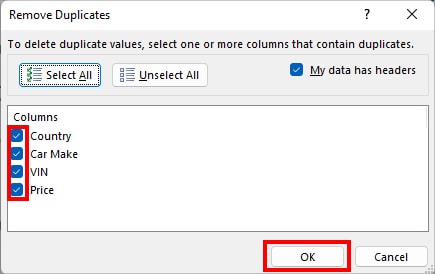
- On the Remove Duplicates window, check all the boxes for Columns with Duplicates. Then, click OK.
Check and Correct the Typo
Unlike other Office programs, Excel does not auto-suggest spellings when there’s a typo. So, either you’d get the formula error or a different result. Also, if you’re sharing an Excel sheet with others, you wouldn’t want them to see incorrect spelling and grammar.
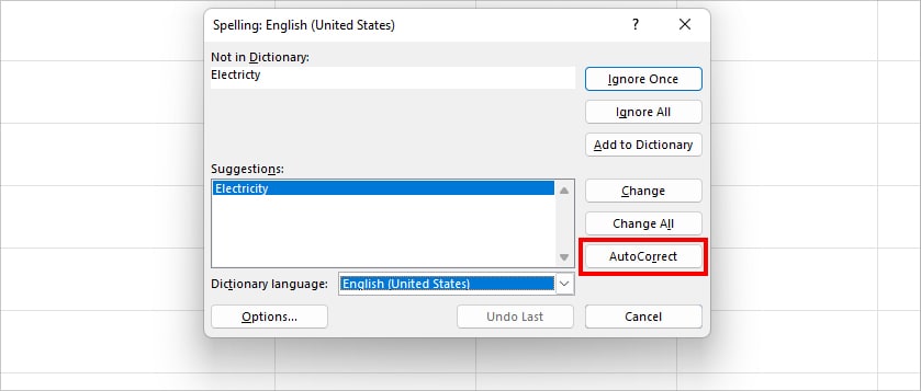
To fix this, select your data and press the F7 key to look for spelling errors. On the Spelling window, you’ll see suggestions. Click the AutoCorrect button to correct them.
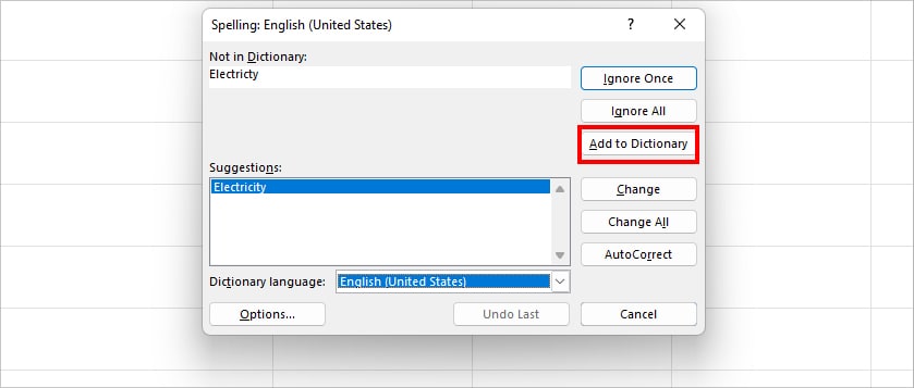
However, you can add the custom word to the dictionaries if needed. For this, click Add to Dictionary button.
Trace Errors and Solve them
Everyone loves worksheets that have no errors.
It is common to get Excel errors when you perform calculations and use formulas. But, if you do not solve them, your worksheet will be full of yellow exclamation marks and errors like #DIV/0!, #VALUE!, #REF!, etc
To deal with different types of errors, you can use the Error Checking tool. It’ll help you identify the exact cause that’s resulting in an error.
- Select the cell with an error and go to Formulas Tab.
- From the Formula Auditing group, click on Error Checking.

- On the Error Checking Window, you can see the cause of the error.

- Now, change the arguments in the formula as required to solve the error.
Change Data Formatting
Knowing how to format the data as per the need is one of the pro tips to keep your spreadsheet tidy. For example, for a date entry, a simple short date might be enough. Long dates with timestamps might be insignificant which will only take up space and result in a #### error.
It’s better to change the format and keep only the necessary information. For this, select your data and go to Home Tab. In the Number section, expand the drop-down menu and choose the format as required.
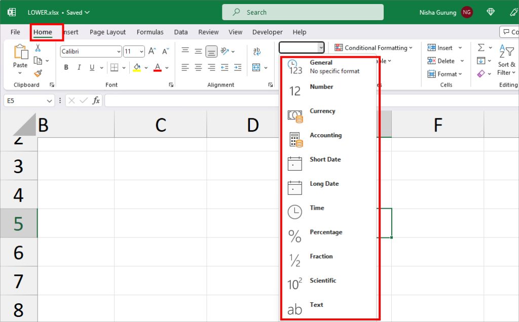
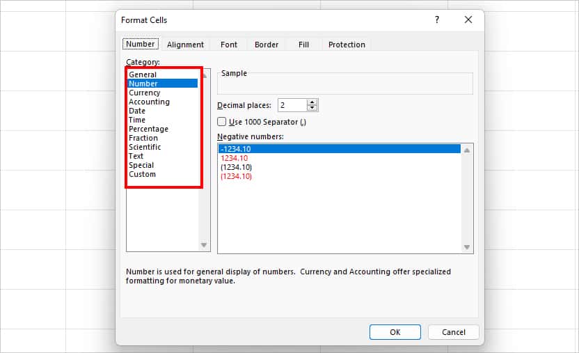
Alternatively, you can find more format options in the Format Cells window. Enter Ctrl + 1 keyboard shortcut to bring up the Format Cells window.
On the Number tab, go to each General, Number, Currency, Accounting, Date, Time, Percentage, Fraction, Scientific, Text, and Special category to explore the formats. If you wish to apply your own custom formats, click on the Custom category and enter a type. When done, click OK.
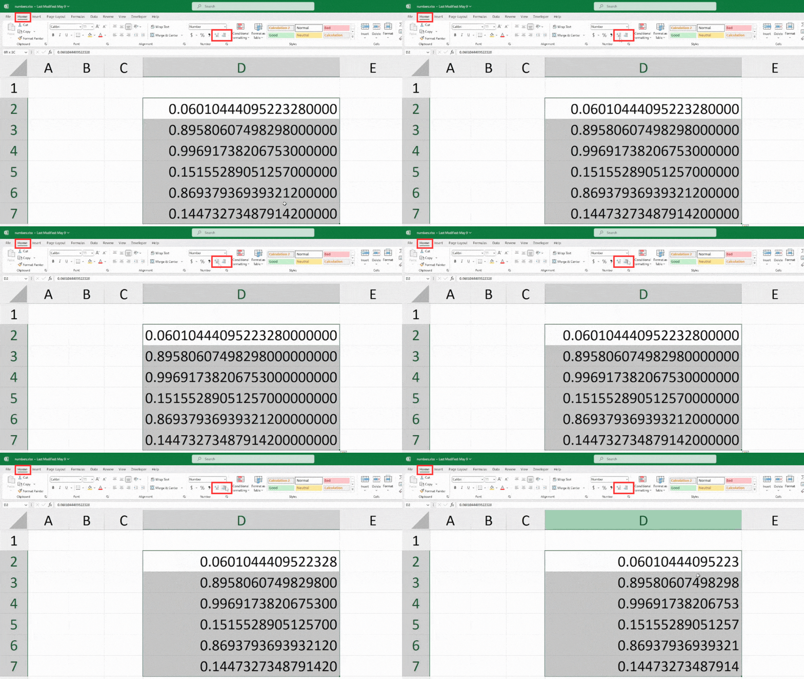
For the Decimal numbers, you can use Increase Decimal or Decrease Decimal of Home Tab to format them. If you do not want your numbers to round up, click on Increase Decimal. But, this will increase the decimal place. However, to have the decimal numbers short and rounded up, click on the Decrease Decimal.
Delete Blank Cells
If there are unwanted blank cells in your spreadsheets, delete them immediately. A blank cell can confuse users to think whether they’ve left intentionally or not.
- On your Sheet, enter Ctrl + A to select all data.
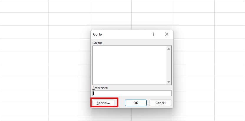
- Press Ctrl + G for the Go To window. Then, click Special.
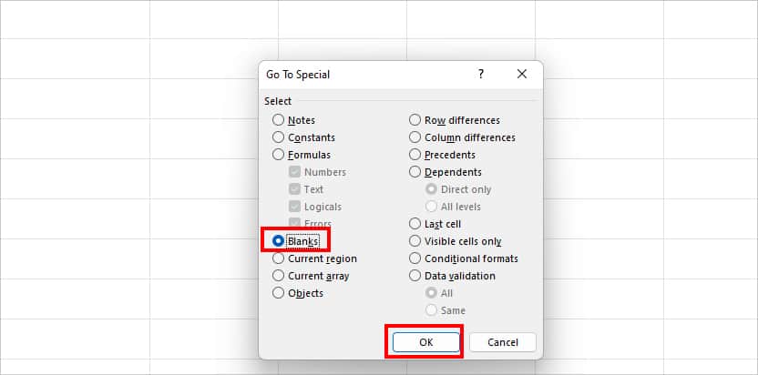
- On Go To Special, click on Blanks and hit OK.
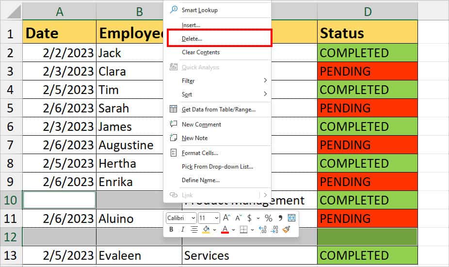
- Right-click on the highlighted Blank cells and choose Delete.
- On the Delete window, choose one of the options:
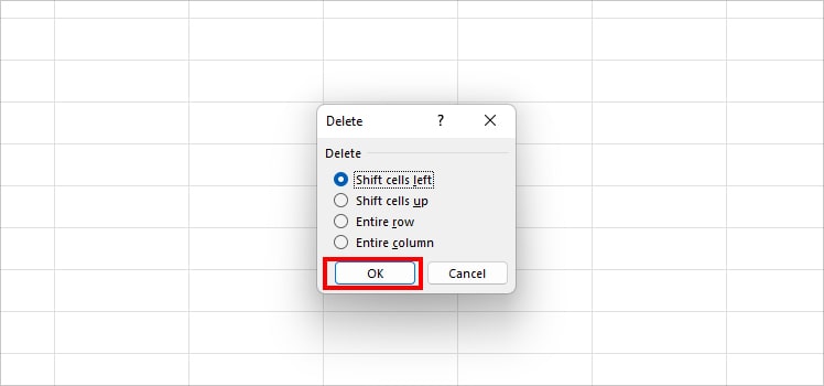
- Shift cells left: Deletes blank cells and shifts the cells to the left.
- Shift cells up: Deletes blank cells and moves the cells up.
- Entire row: Deletes all rows with blank cells.
- Entire column: Delete the whole column containing blank cells.
- Click OK.
Delete Unnecessary Rows and Columns
When dealing with huge data in a worksheet, it isn’t necessary that all of the rows and columns are useful. Sometimes, you may have created a helper column as support to input the formula. Or, it could be just the unused rows and columns. Nonetheless, if you have such rows and columns, it’s best to delete them.
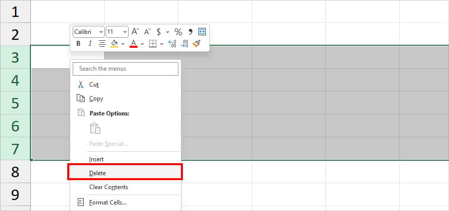
- While pressing down the Ctrl key, select the multiple Rows or Columns.
- Right-click on the selection and choose Delete.
Split Columns
If your column contains numbers and letters all jumbled up in one place, your spreadsheet can look very chaotic. In that case, you can split columns with street addresses, separate names, names and numbers, etc. For this, you can use Excel’s Text to Columns feature.
As a basic example, let’s split the column with Street Addresses.
- Select the cell ranges.
- Go to the Data Tab. From Data Tools, click on Text to Columns.
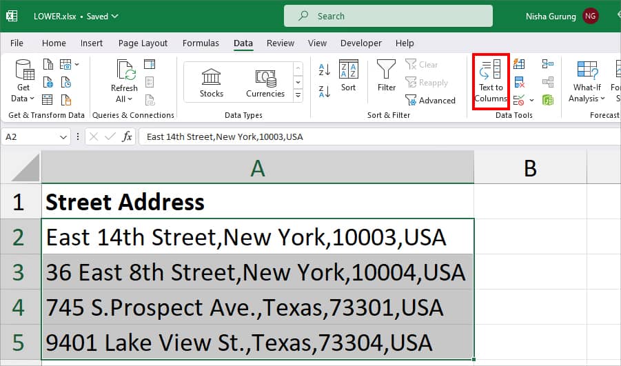
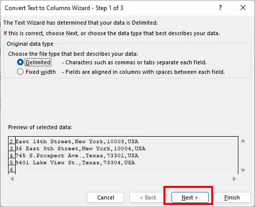
- On Convert Text to Columns Wizard window, choose Delimited and click Next.
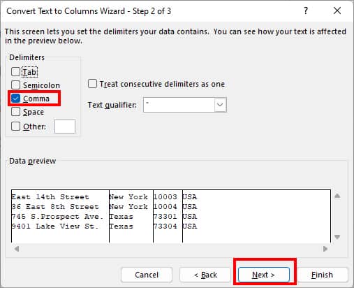
- On Delimiters, untick the option for Tab. Then, check the box for Comma and hit Next. (Our data is separated by comma)
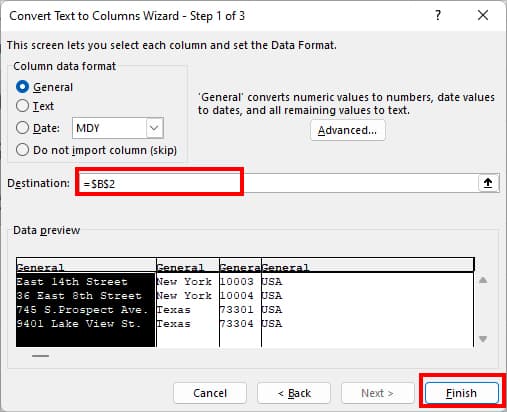
- On Destination, choose a Cell to import data. When done, click Finish.
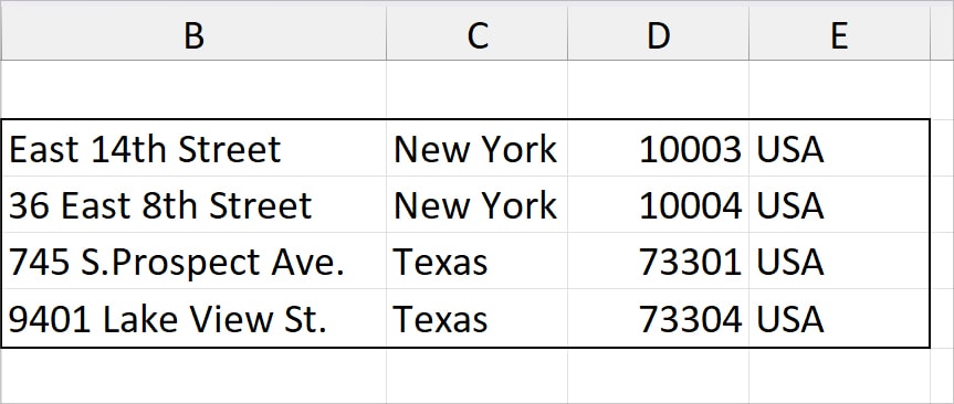
- You’ll have Addresses in different columns.
Merge Cells or Columns
Separating the columns does not always mean you’ll have a systematic worksheet. If the values are unnecessarily split all over the columns, it can look unorganized. For example, having names in one column and domain addresses in another column will only increase the column size. During such cases, it’s better if you merge the columns.
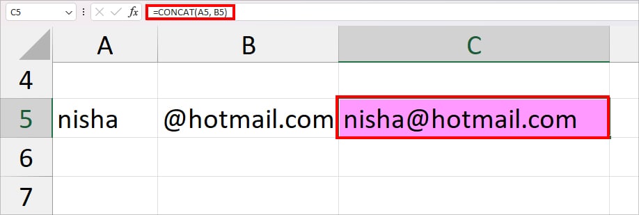
To combine columns, you can use the CONCAT function. CONCAT function joins the two or more values you pass down in the formula together.
See this example to use the CONCAT function. We have the person’s name in Column A and the domain address in column B. If you enter =CONCAT(A5,B5), the formula returns [email protected].
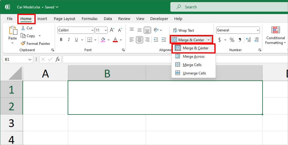
Now, another case where merging cells work best is if you have large heading texts. I prefer using this when I do not want to expand the entire columns for a single text. To do so, select the Cell ranges and go to the Home tab. From the Alignment section, click on Merge & Center > Merge & Center.
Customize Page Setup
If you need to print Excel spreadsheets, you need to take care of what the print page looks like. Although the worksheet looks organized, it may not appear as you expected on the print page. This could happen when the print page spans and your information is divided into two or more pages. To avoid this, there are a few print setup settings you can configure as per required.
- Open Excel workbook and go to the Page Layout Tab.

- On the Page Setup group, click on the Dialogue Launcher.

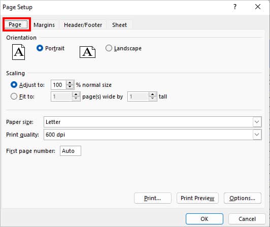
- On the Page Setup window, head to Page tab to set page Orientation, Scaling, Paper size, Print quality.
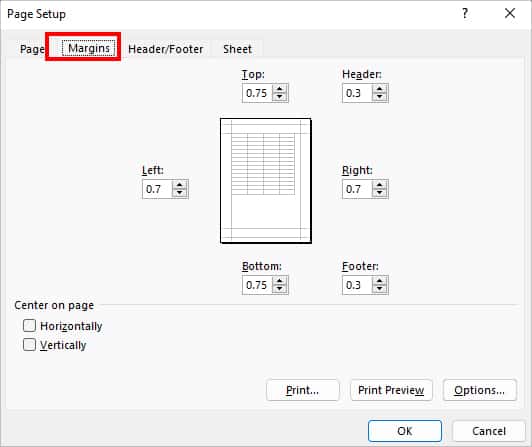
- Go to the Margins tab and adjust the Paper Margin.
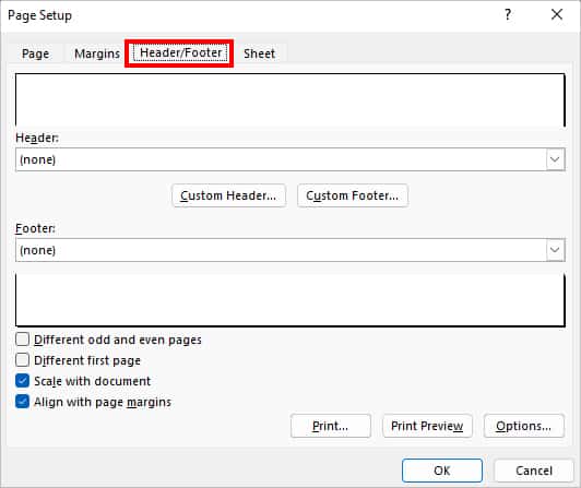
- Now, click on the Header/Footer tab to add Header and footer.
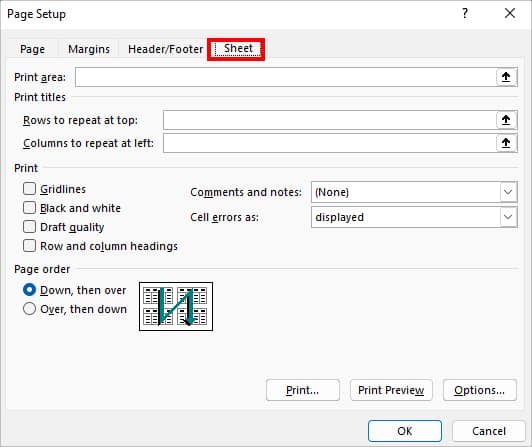
- Finally, go to the Sheet tab to set the Print area, Print titles, Page order.
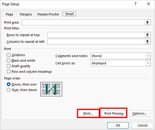
- Click on Print Preview to see the page. Or, hit the Print button.
ProTips to Keep Your Data Clean in Excel
By now, you must have learned how to clean data on your existing filthy spreadsheet. But, there are possible chances that you may have a similar worksheet in the future, right?
Here’re some of the tricks I personally follow to maintain my spreadsheet. You could also learn some of these to avoid having dirty spreadsheets.
- For any kind of data entry, create Excel’s Data Entry Form. You can record information of an entire row at once.
- I recommend you use the F7 key more often to check spelling.
- Identify appropriate Cell Styles to highlight your information in cell values. For Instance, if you have a formula cell, it’s better to use a Calculation style rather than an Input cell or Check Cell.
- I know Conditional Formatting has a lot of options to highlight cells based on a particular condition. But, don’t overdo it. Try to apply formats only in the required cells.
- Apply Borders for a clear division of cells on your spreadsheet.
- If you’re unsure of your formatting, apply pre-built themes such as Slice to make your spreadsheet look decent yet professional.
- It’s better to separate large-row lists with commas and have them in one row.
- Delete unused columns, unwanted spaces, duplicates, blank cells, etc. Try to make your worksheet as informative as possible.
- Immediately solve formula errors on your sheet.