How to Add Text to Columns in Excel

Although data entry is done best on a spreadsheet, you may sometimes receive data as text. It can get quite inconvenient to manually enter information in individual columns. To overcome this, Excel has a special feature called Text to Columns.

Text to Column is a dedicated Excel feature to convert text into individual columns. Even though the application of this tool is quite simple, your approach may differ depending on your text. Similarly, this tool could be limited for more advanced conversion. In such cases, you can always head to the Power Query to split your text into columns.

In this article, we’ve used four examples to help you understand how you can add text to columns in Excel using the Text to Column utility.

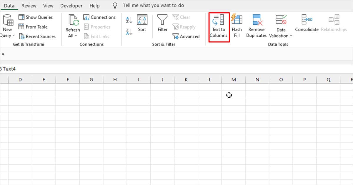
Firstly, let’s discuss where you can find the Text to Columns tool.

1. Open your Excel workbook.
2. Head to the Data tab.
3. Locate Text to Columns in the Data Tools section.
   

Case 1: Text is Separated by Space

Most text data are usually separated by space. You can use the space between your text as a separator to break text into columns. 

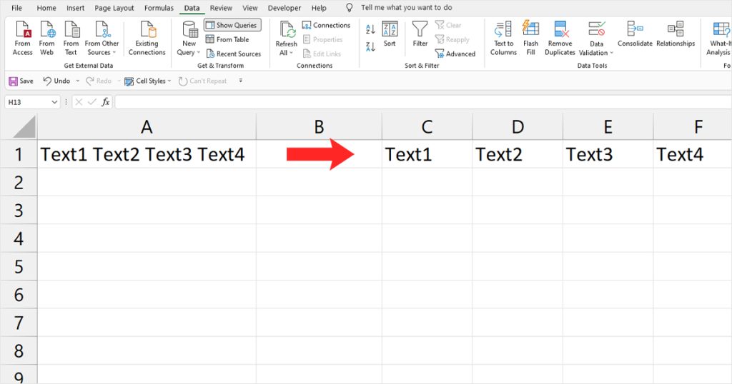
In this example, we have our text separated by a space. You will have to set your separator as space in this case.

1. Open Text to Columns.
2. In Step 1 of 3, select the box next to Delimited, then select Next.
   
3. In Step 2 of 3, choose Space under Delimiters > Finish.
   

As a result, we have all four of our characters in four separate columns. If your text is separated by other characters such as commas, semicolons, or anything similar, simply enter the symbol in Step 2 of 3 of the Text to Column wizard.

Case 2: Text that Follows a Format to Column

Let’s take for instance: you’re entering data from a form into individual columns. As forms usually follow a format, you can use that as an advantage to separate text into columns.

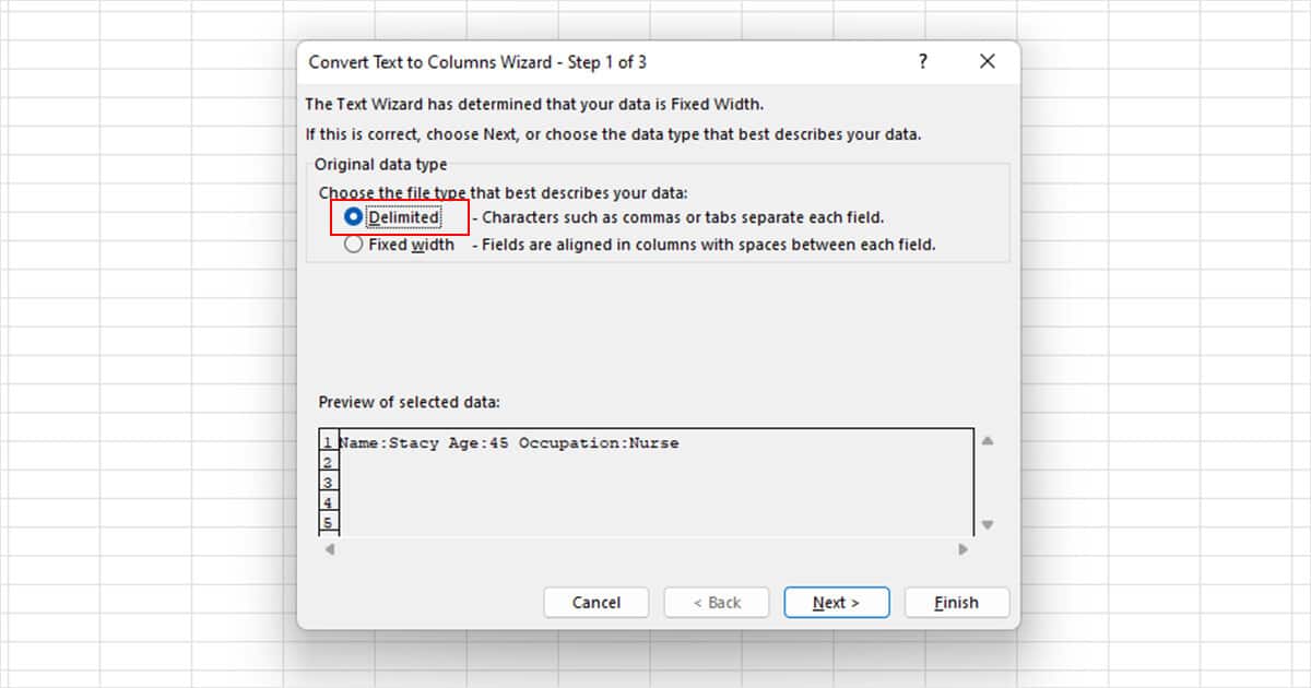
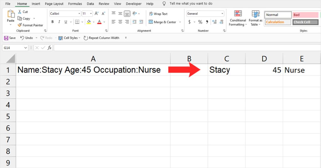
For this example, we’re looking to separate “Name:Stacy Age:45 Occupation:Nurse” into three columns.

1. Select your text in the grid and open Text to Columns.
2. In Step 1 of 3, select Delimited > Next.
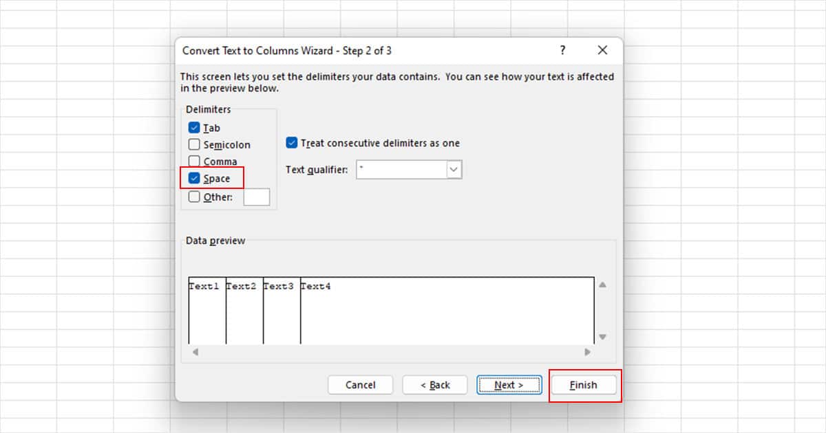
3. In Step 2 of 3, choose Space > Finish.
   
4. Once you exit Text to Columns, use Ctrl + H to open Replace window.
5. Next to Find what, enter *:
   
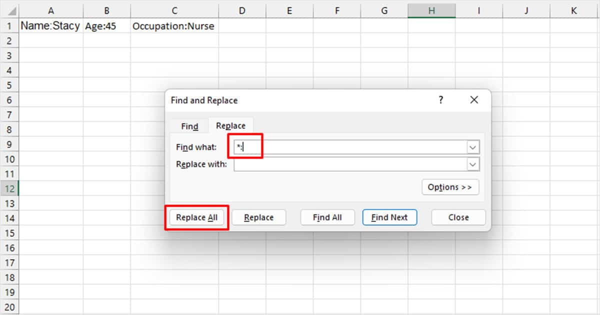
6. Leave the Replace with section empty.
7. Click the Replace All button.

The Find and Replace tool in Excel supports wildcards such as the asterisk sign. What the asterisk does in this context is, it selects all data entered before the colon sign. As Name, Age, and Occupation preceded the colon sign, they were removed using the command.

Case 3: Text is Not Separated but is in Camelcase

Another likely situation you may encounter is if your text comes without spaces between them. You will have to use Power Query to separate text as such into columns.

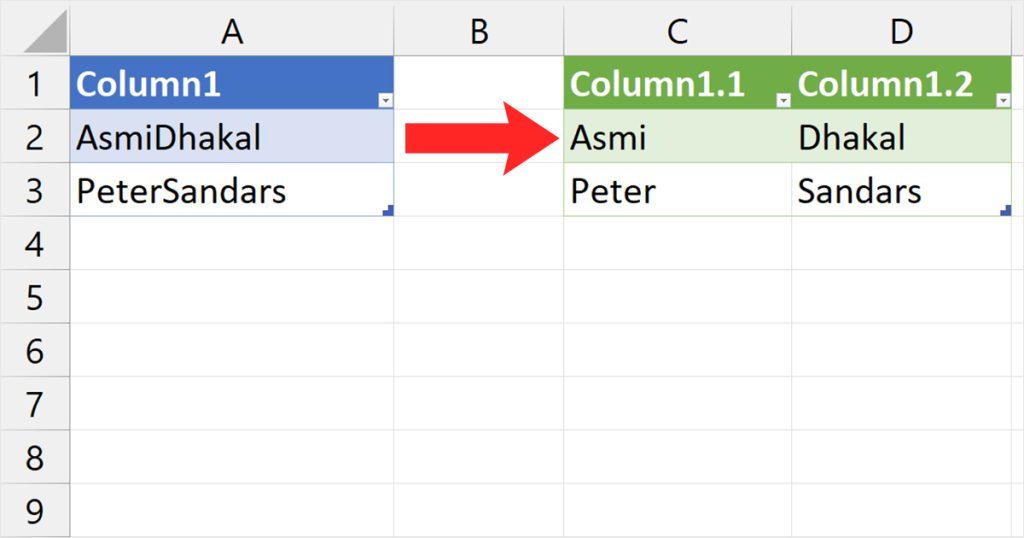
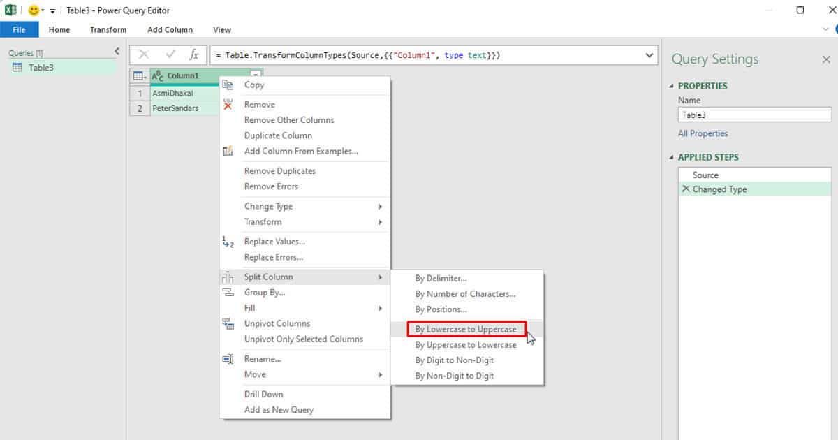
Here, we’re looking to separate the name, AsmiDhakal. The text has no space in between, but the initials of the first and last names are in capital letters. You can also use this method to separate multiple texts into columns at the same time.

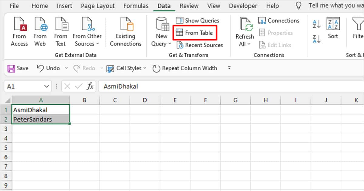
1. Select your cell or range, then head to the Data tab.
2. From the Get & Transform section, select From Table.
   
3. In the Power Query editor, right-click on the column header.
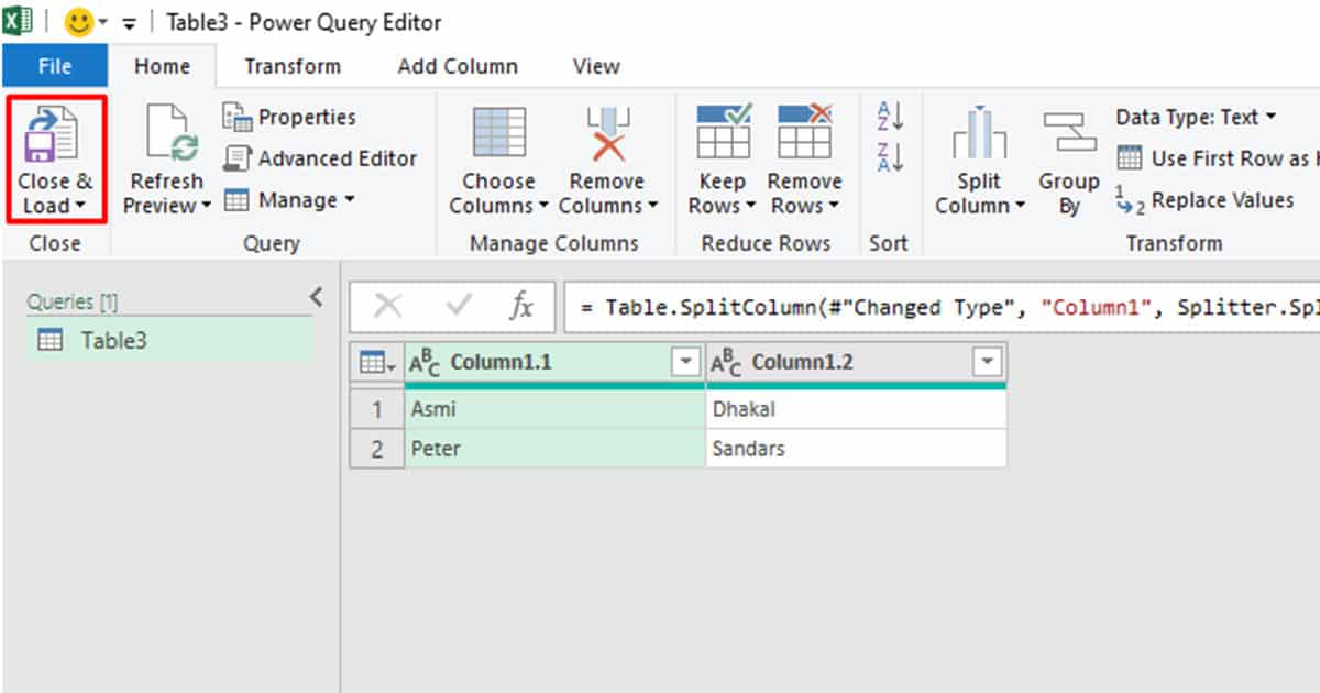
4. From the fly-out menu, head to Split Column > Lowercase to Uppercase.
   
5. Select Close and Load on the home tab.
   

Case 4: Separate String Values

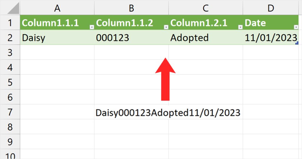
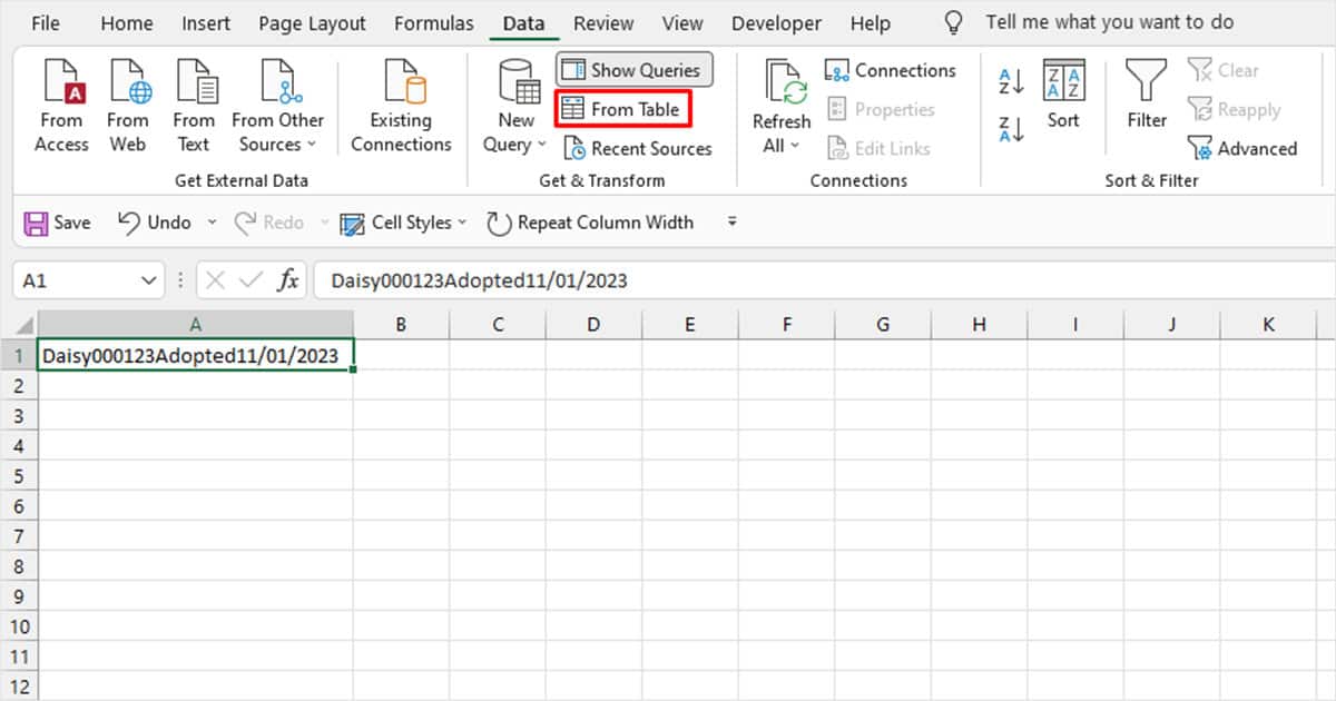
For this occurrence, let’s assume you’re working with a report. The report is on the status of animal rehabilitation for five dogs. In your report, you need the Name, ID number, Status, and Date of Rehabilitation.

Separating string values may come off as a bit tricky given that you’re dealing with both text and numeric values. However, Power Query has a dedicated feature to separate such values into columns.

For this situation, we have divided one method into three steps for better retention.

Step 1

1. Select your data from the grid and head to the Data tab.
2. In the Get & Transform section, select From Table.
   
3. Right-click on the column, and select Split Column > Digit to Non-digit.
   

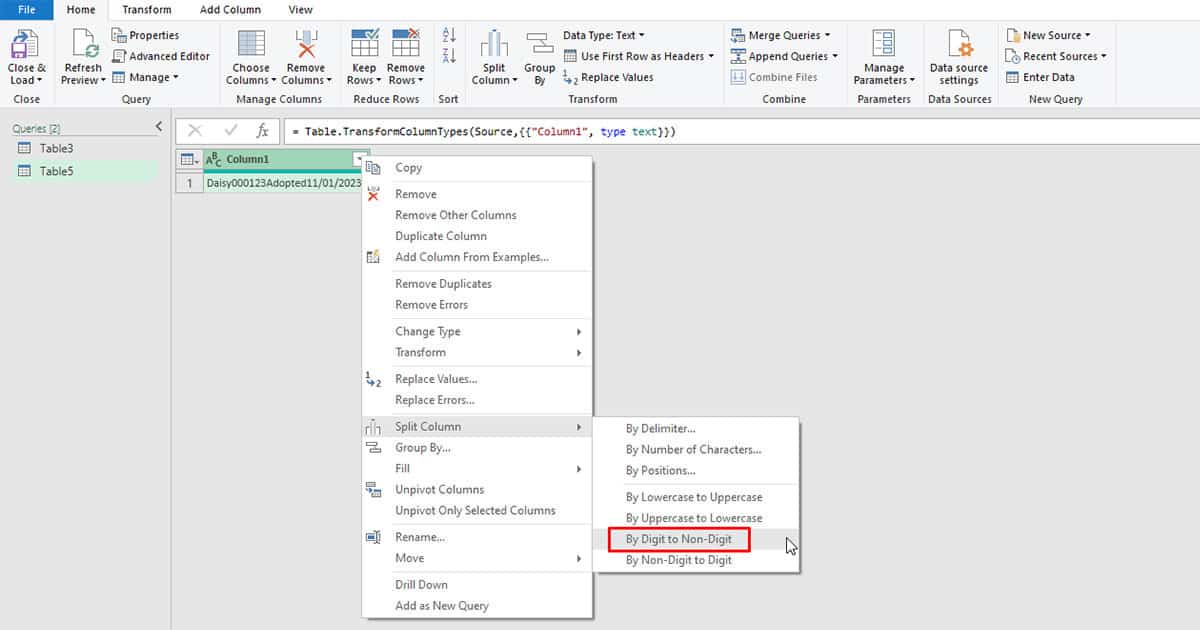
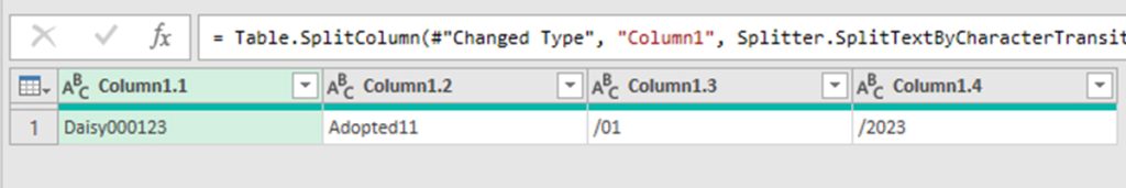
In the first step, we used Digit to Non-digit to divide our row into four columns. The split column tool looked for a digit in our value and if a non-digit followed, the text was separated it into individual columns.

Step 2

1. Right-click on column 1.1.
2. Select Split Column > Non-digit to Digit.
   
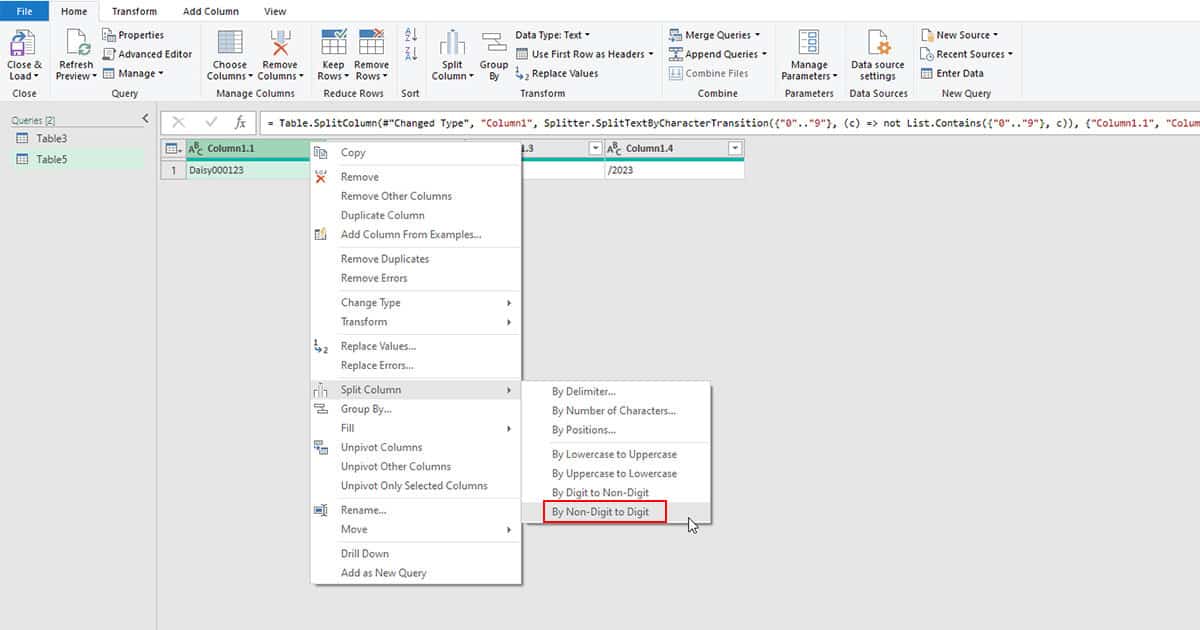
3. Repeat this for column 1.2.

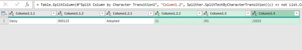
Heading on to step 2, we further segregated columns 1.1 and 1.2 into four individual columns. We use Non-digit to Digit in this scenario to split “Daisy”, and “000123” in column 1.1, and “Adopted”, and “11”.

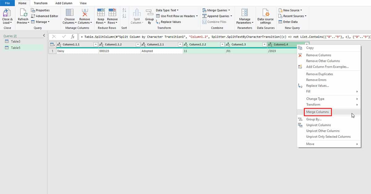
Step 3

1. Click on column 1.2.2, hold Shift, and select column 1.3 and column 1.4.
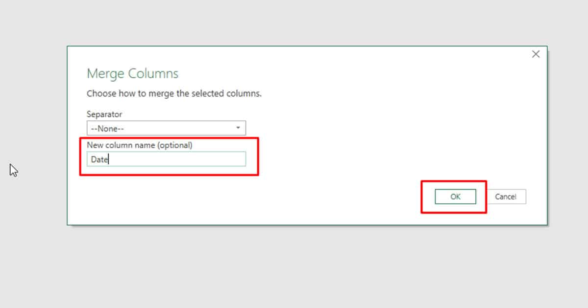
2. Right-click on any column header, and select Merge Columns.
   
3. In the Merge Columns window, rename your column and click OK.
   
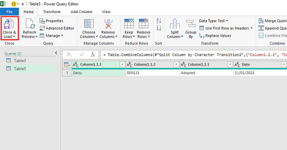
4. Close and Load your data from the Home tab.
   

Now that we’re done splitting our text, let’s do some merging. If you’ve noticed, using Digit to Non-digit in step 1 separated “11/01/2023” which is our date. After Step 2, “11”, “/01”, and “/2023” are placed into individual columns. To place them in one column, we used the Merge Column tool with no separator selected.