Filter Not Working? Here’s How to Fix It

Is your Filter tool greyed out? Or, is it not applying a Filter to all of your data?

Well, these are the most two common issues users face when using this tool. But, mind you, the issue is temporary and is solvable with basic fixes. 

Before we dive into the fixes, let’s quickly see what causes the filter to not work.

Preliminary Check 

First of all, here’s a quick preliminary check you can do. 

1. Is your cell in Editing Mode? When you double-click on the cell to edit contents, Excel greys out the Filter Menu.
2. Check if you have selected multiple Sheets or Grouped sheets in your workbook. In this scenario too, you will see that the Filter button is greyed out.
3. Have you selected cell ranges to apply the filter? To use the Filter, simply selecting one cell within the table/data is enough. 
4. Have you assigned the (Ctrl + Shift + L) Filter keyboard shortcut for other commands? If the (Ctrl + Shift + L) to turn On/Off the Filter button is not working, it’s possible another command has overridden the shortcut. 

How to Fix Filter Not Working in Excel?

Check Format and Convert If Needed

When using the Filter, it is important you have the data in the appropriate format. For example, if your dates are formatted as texts, you won’t see the date filter with separate Months, Years, and Days. Same is the case for currencies and numbers.

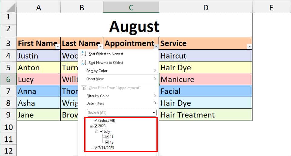
If your Filter tool is working fine, but not filtering the data as expected, there’s definitely a problem with the data format. To fix this, you can check and change as required. 

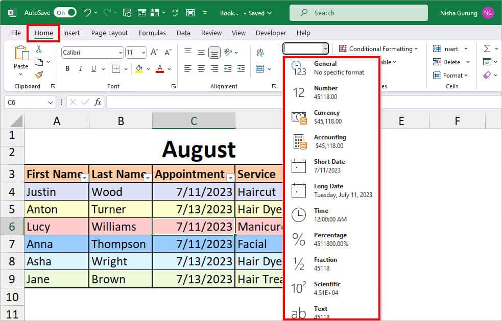
For this, select your Column and go to the Home Tab. On the Number group, expand the Drop-down menu and choose the right Format for your data type. 

Resize Table and Reapply Filter

In Excel, you can apply the Filter only once at a time. And to AutoFilter your entire data, you must make sure the data is contagious. If you have added the columns or rows which are not adjacent to your last table, you won’t see those values in the Filter. Basically, in short, Filter will work for only partial data like in the picture. 

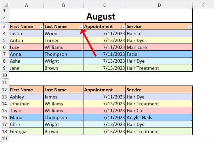
In that case, you can extend the Table range and reapply the filter. This fix has solved the problem for many users. 

1. Select any cell within your table and press Ctrl + Shift + L to Remove Filter.
2. Go to the Table Design tab and click on Resize Table.
   
3. On Resize Table, use the Collapse icon to select the Entire data in your worksheet. Then, click OK.
   
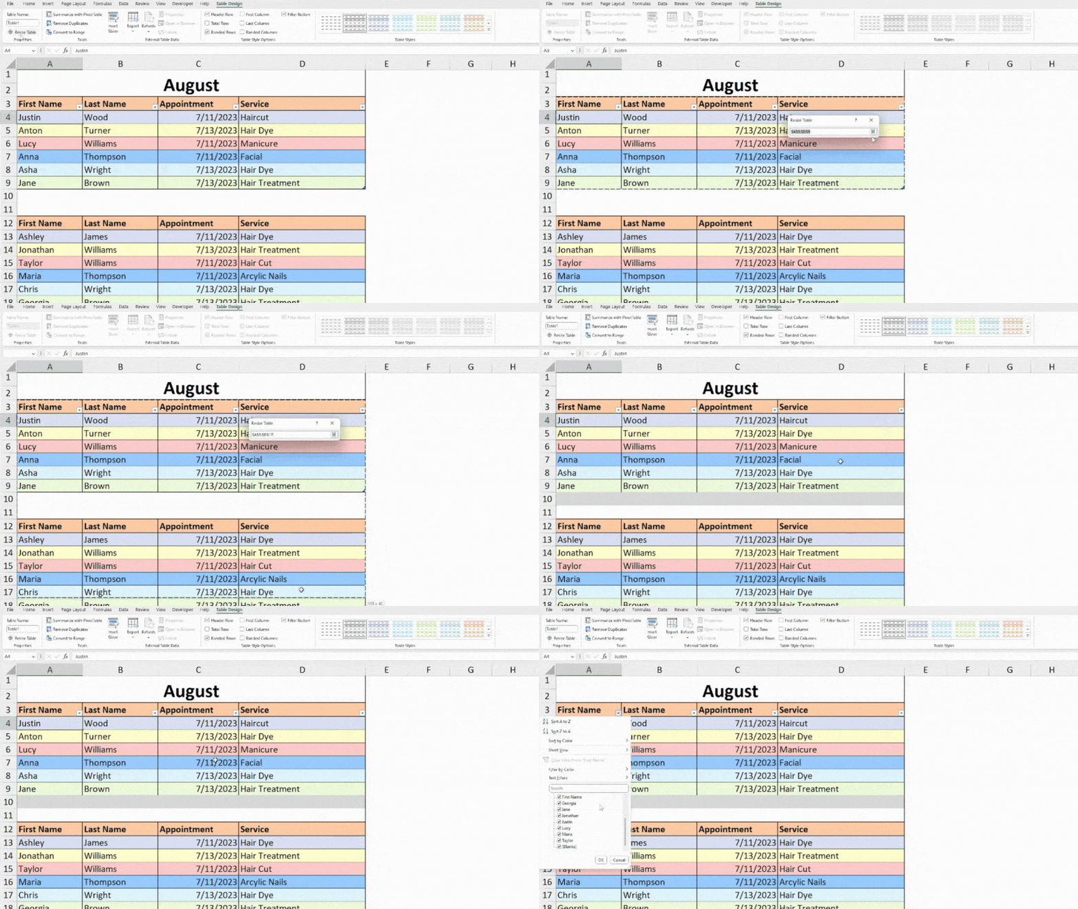
4. Now, click any Cell in your table and enter Ctrl + Shift + L shortcut key to turn on the Filter.

Delete Blank Rows

As we’ve mentioned earlier, Excel does not apply the filter to data that are non-contagious. If you have blank cells or rows in your sheets, Excel will not select the ranges past them. Especially, if the data is not formatted as a table. To address them, you can delete the blank rows.

1. Select the entire data. 
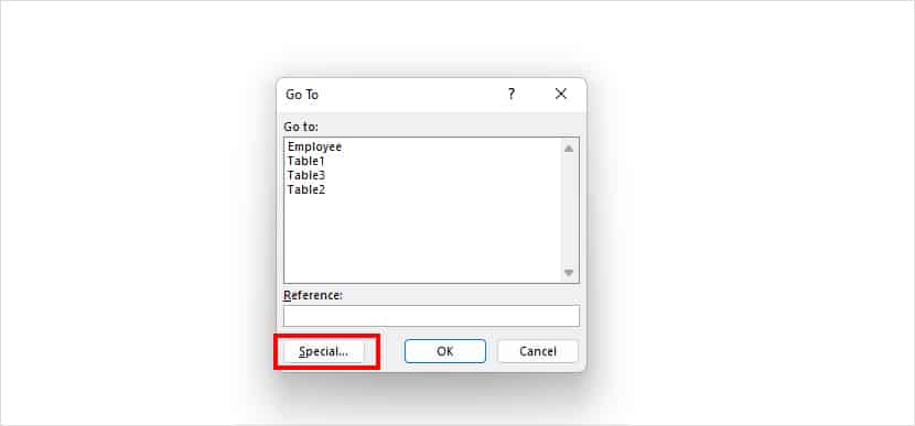
2. Enter the Ctrl + G shortcut keys for the Go To Special window. Then, click Special.
   
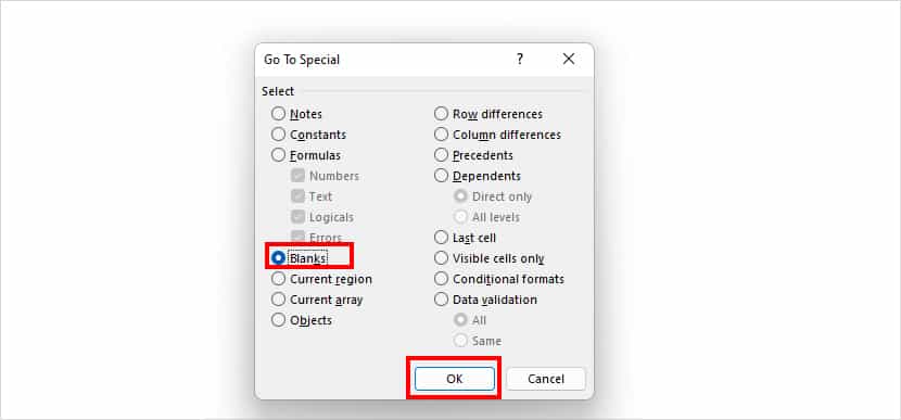
3. On the window, choose Blanks and click OK.
   
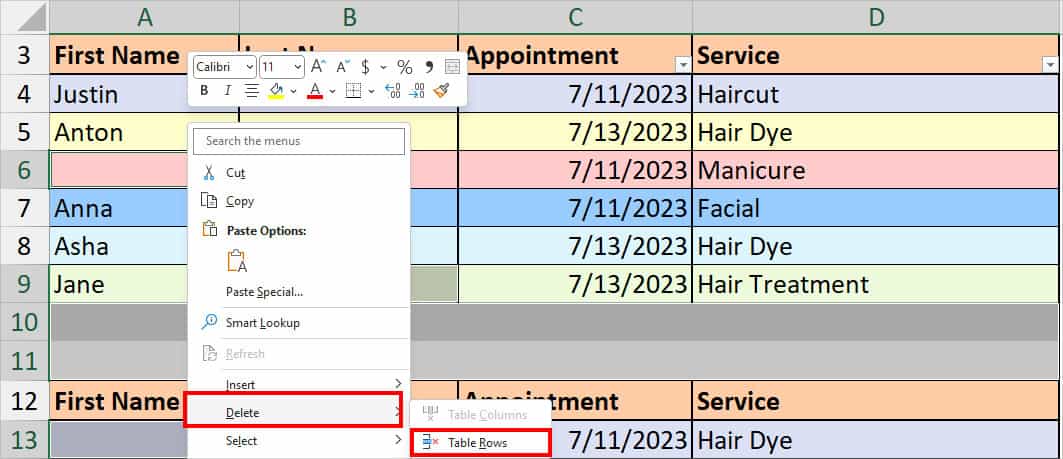
4. Right-click on any one selected Blank cell. Pick Delete > Table Rows.
   

Unmerge Cells

While Excel’s Merge and Center feature comes in handy to combine cells into one, it can be just a hurdle when using the Filter. This is because you‘ll only have the top-left value in the cell with the rest of them discarded. It could be one of the reasons the Filter tool is not filtering your values as intended. 

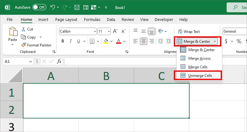
Using Ctrl + A, select your data. From the Home Tab, click on Merge & Center in the Alignment section. Choose Unmerge Cells. 

Unhide Columns and Rows

If you have noticed the Filter tool has excluded certain values, it’s probably because the rows or columns are hidden. It is impossible to track down the hidden ranges manually by yourself in large spreadsheets. So, you can unhide them.

1. From the top-left of your Sheet, click the Select All button.
   
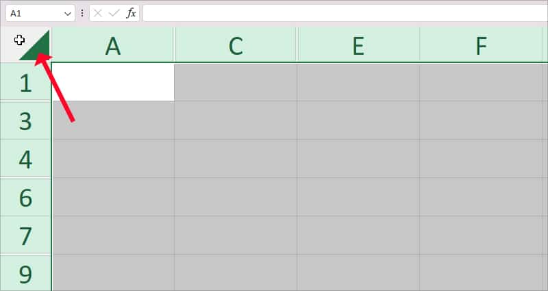
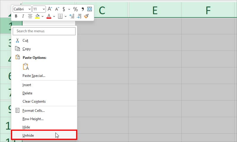
2. Right-click on the Row Header. Then, choose Unhide in the fly-out menu.
   
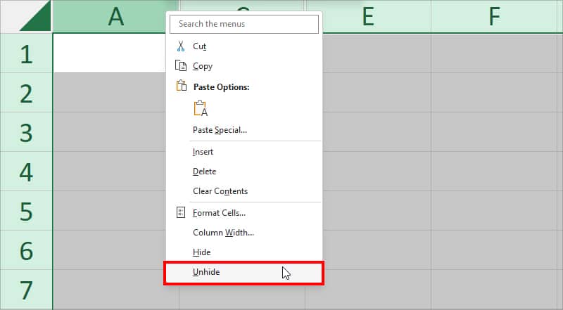
3. Again, hover over the Column Header. Right-click on them and click Unhide.
   

Unprotect Sheet

If you’re working on a password-protected sheet, it could have a lot of restrictions. You’re lucky if the user has allowed you to use the AutoFilter. However, even if you could filter data with the criteria, you still won’t be able to turn on or disable the Filter.

Now, for users who do not have access to AutoFilter, Excel will grey out the Filter menu in the ribbon. Although you may see the Filter button, it won’t show the item lists. To fix this, you can Unprotect Sheet if you know the passcode.

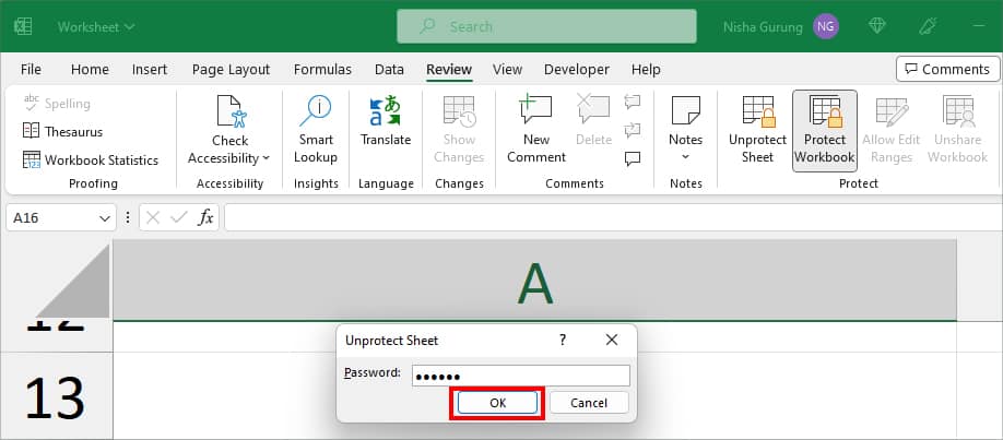
1. Go to the Review Tab.
2. Click on Unprotect Sheet.
   
3. If prompted, type in the Sheet Password and click OK.
   

Repair Office

By now the problem should have been solved for many users. But, if the Filter is still not working, there could be glitches and bugs in the app. In that case, you can Repair Office yourself. It will automatically identify the error and troubleshoot them.

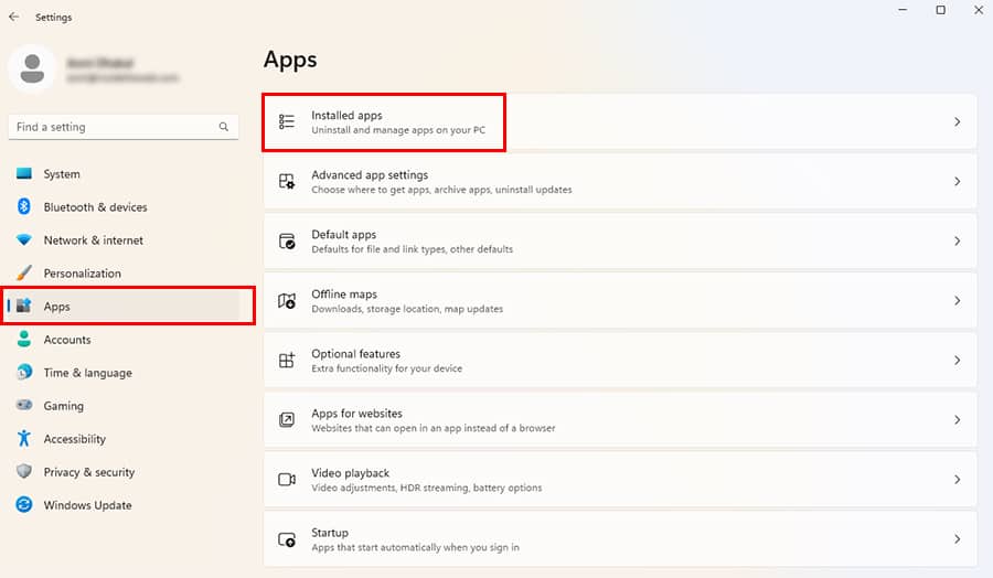
1. For Windows Settings, press down Windows + I.
2. Navigate to Apps > Installed Apps.
   
3. Now, hover over the Office app or Microsoft 365 app. Click the More icon and choose Modify.
   
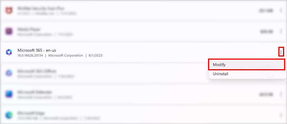
4. On the prompt, choose Yes.
5. On Microsoft Window, pick Online Repair. Hit Repair.
   
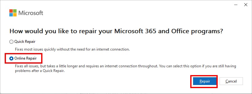
6. After the repair, Restart your device. Launch Excel and try using Filter again. 

Update Office

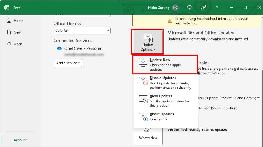
If repairing the app didn’t fix the problem, update the app with the latest software version. Buggy software can only be fixed by upgrading to a newer version. The official team might have released bug fixes in the recent updates.

1. Launch Excel.
2. Click on Account.
   
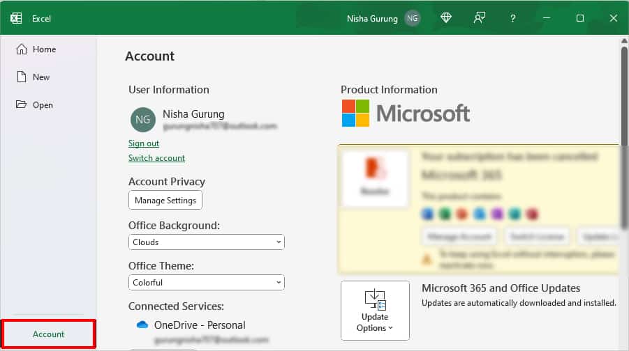
3. Select Update Options > Update Now.
   

Use FILTER Function as Alternative

In case, none of the fixes work, use the FILTER function as an alternative. The FILTER function is built to filter out the values based on various criteria. Compared to the tool, it has more advanced features. Also, the function is beginner friendly.