Sometimes, you might need to compare two columns to pinpoint the missing values, detect the same match, find unique items, and so on.
If you think the VLOOKUP function can take just one lookup table in the formula, you aren’t using it at its full potential. Meaning, you can use the two ranges of columns in the VLOOKUP by nesting them with another formula.
Here, I will cover all the examples of using the VLOOKUP to compare columns in both the same and different workbooks.
Compare Two Columns in the Same Sheets
Check out these 4 examples to compare two columns in the same sheet.
Example 1: Find Missing Value
Suppose, I have lists of car names in Columns A and C. I want to check whether the car in Column C is missing from Column A.
To find out, I will simply use the VLOOKUP formula with the exact match as I would normally.
Use the Auto-Fill handle to check in all columns. Remember to use the absolute reference for the range as given below.
Formula:
=VLOOKUP(C3, $A$3:$A$17, 1, 0)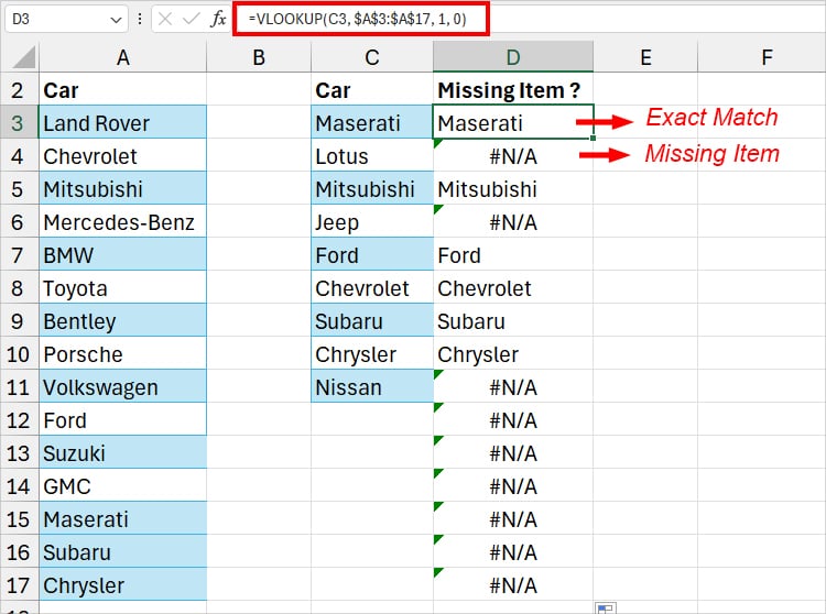
In the VLOOKUP formula, the lookup value is the item in Column C. The ranges in Column A, $A$3:$A$17 is my array, and column 1 is index to return the value from. Similarly, 0 signifies an exact match.
In the output cell, I will either have a car name or #N/A. Also, don’t worry about the #N/A error! The cell with an error means that there’s a missing item.
Address the #N/A error in the Missing Item
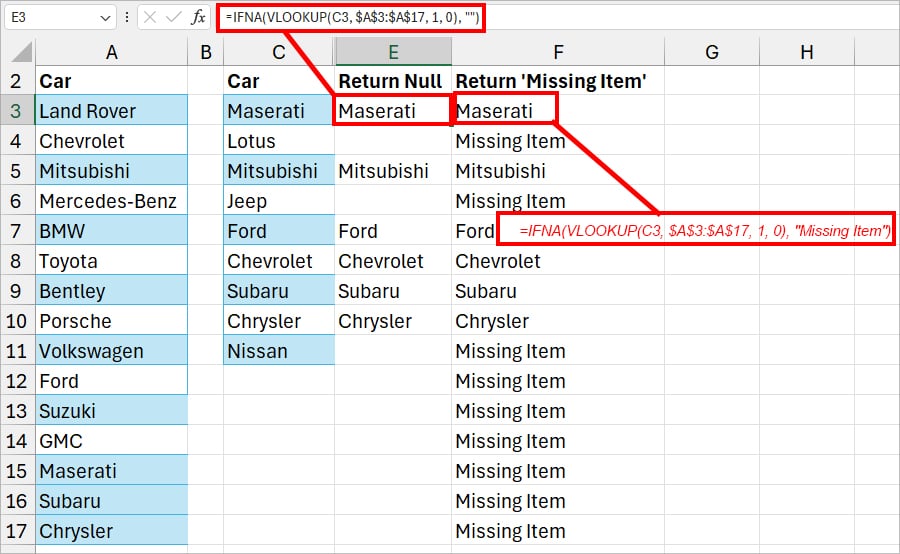
If you don’t want your sheet to be cluttered with #N/A errors after locating the missing item, you can use the IFNA function to ignore it. You could either return a null string making it an empty cell or choose to result in the text string.
Here are some examples. Use the formula and Auto-Fill.
| Example | Formula | Description |
| Return Null | =IFNA(VLOOKUP(C3, $A$3:$A$17, 1, 0), “”) | By nesting the IFNA function in the VLOOKUP, we specified the formula to result in the null string. |
| Return “Missing Item” | =IFNA(VLOOKUP(C3, $A$3:$A$17, 1, 0), “Missing Item”) | The IFNA Function checks for #N/A error in the VLOOKUP output and returns Missing item found. |
Example 2: Find a Similar Item
Suppose, you want to know and extract only matching values from both columns. For that, we will nest the VLOOKUP with IFNA and FILTER functions together.
This time I have converted my range into the Table Format so that it becomes dynamic in the formula. By doing so, I wouldn’t have to worry about changing the cell array in the formula every time. Also, to make it easily distinguishable, I have named those tables.
Formula:
=FILTER(CarOne[Names],IFNA(VLOOKUP(CarOne[Names],CarTwo[Names],1,0),"")<>"")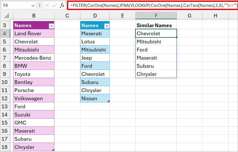
The formula returned an array of names that lie in both Columns B and C.
Formula Breakdown:
- IFNA(VLOOKUP(CarOne[Names],CarTwo[Names],1,0),””): Here, our lookup value is the entire Column of the second table (CarTwo[Names]) and array to return 1 index is Table 1(CarOne[Names]). The formula returns null for #N/A and names for the exact match.
- FILTER(CarOne[Names],IFNA(VLOOKUP(CarOne[Names],CarTwo[Names],1,0),””)<>””): Finally, the FILTER function eliminates the empty cells with disguised error and returns only the matches.
Example 3: Find a Different Item
Now, let us move on with the formula to check both columns and return a different item.
To extract the unique names by comparing two columns, I will construct the formula nesting the FILTER, ISNA, and VLOOKUP together.
Formula:
=FILTER(B4:B18, ISNA(VLOOKUP(B4:B18, D4:D12, 1, 0)))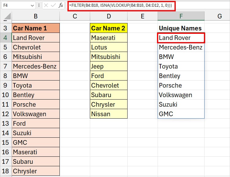
The formula returned an array of Unique Car names.
Formula Breakdown:
- VLOOKUP(B4:B18, D4:D12, 1, 0): The VLOOKUP returns the matching names from Car Name 1 and Car Name 2 Column. For no match, I got #N/A error.
- ISNA(VLOOKUP(B4:B18, D4:D12, 1, 0)): ISNA function returns TRUE for cells containing an error and FALSE for text items.
- FILTER(B4:B18, ISNA(VLOOKUP(B4:B18, D4:D12, 1, 0))): Finally, the FILTER function includes only TRUE cells from the B4:B18 range, resulting in unique names only.
Example 4: Find Partial Match
When using VLOOKUP to compare two columns, elements like correct spellings, spaces, full names, etc matter a lot.
For Instance, if I have BMW X5 in Column A and X5 in Column B, VLOOKUP will result in #N/A. So, instead of performing an exact match, you could also do the partial match using the wildcard entries.
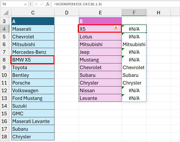
Formula:
=VLOOKUP("*"&E4&"*", $C$4:$C$18, 1, 0). 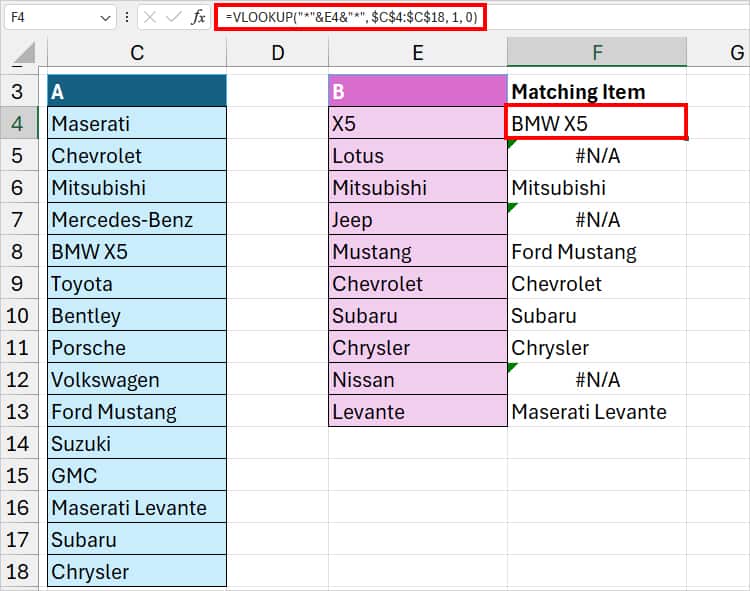
The VLOOKUP formula finds the partial match of Column B in Column A and returns the values. This time for our lookup value, we have used the Asterisk (*) wildcard and concated it with the Ampersand symbol. Using the Auto-Fill handle, drag the formula to all columns.
So, for the first value of X5, it looked for texts that contain X5 whether it’s in the beginning or end. However, in case there are no matches, it returns #N/A.
Compare Two Columns Across Two Sheets
Sometimes, you may want to compare the columns that are in different sheets. Here’s how you do it.
Example:
I have car name data in Column B of List1 and List2 sheets. I want to check and return the matching items in List2 and for #N/A return “Missing Name.”
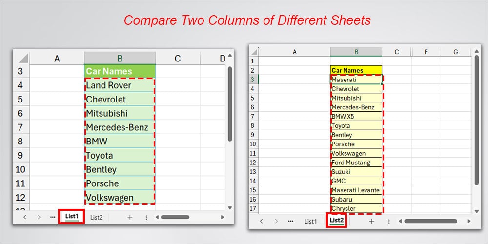
Formula:
=IFNA(VLOOKUP(B3,List1!$B$4:$B$12,1,FALSE), "Missing Name")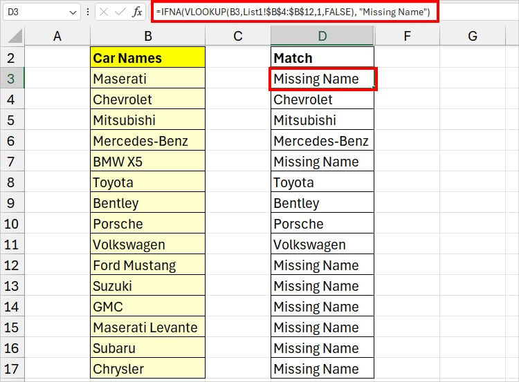
After you get the result, copy down the formula. The formula returned the names for exact match and Missing Names as a result. Here, our lookup value is cell B3 in the List2 sheet.
For Missing Name, you can either enter the data or highlight the cell to easily separate them in the sheet.
If you’re new to using sheet referencing, I suggest you check How to Do a VLOOKUP Between Two Sheets to delve deeper into it.
Compare Two Columns in Different Workbooks
If you have columns in separate workbooks, use the given formula to compare and extract the required item.
Example:
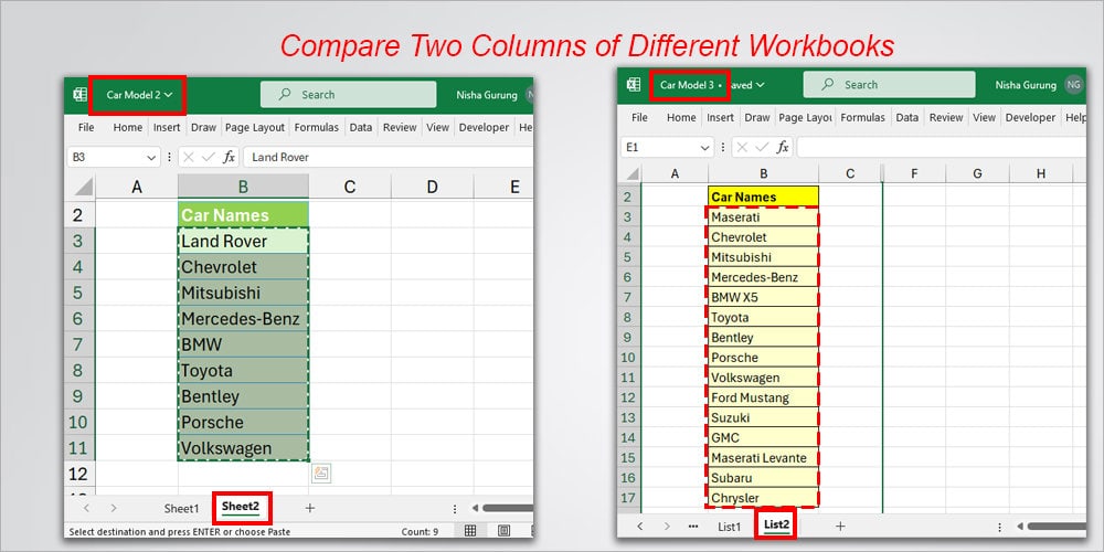
Let’s assume I have Car Names in the Sheet2 of Car Model 2 and List2 in the Car Model 3 workbook.
Formula:
=IFNA(VLOOKUP(B3,'[Car Model 2.xlsx]Sheet2'!$B$3:$B$27, 1, 0), "")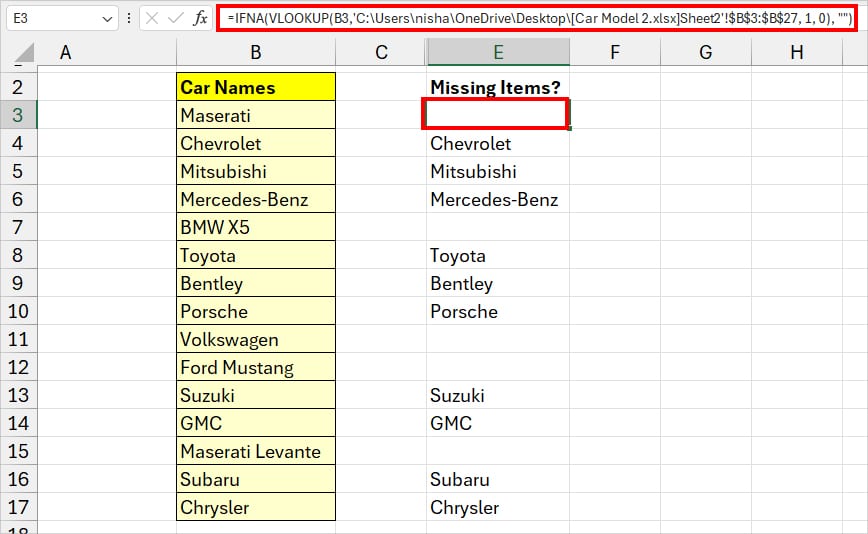
This time, our lookup value is the B3 cell of the Car Model 2 workbook. In the formula, we have specified to return the exact matching names.
Similarly, for the #N/A, we have used IFNA to return a null string and display it as a blank cell.