Over the years, Excel’s VLOOKUP function has been the most popularly used function in Lookup Tables.
The VLOOKUP function returns an exact or nearest match from the Column of a Table range. This function is so powerful that you can also extract value from the lookup table of different sheets or workbooks.
Apart from just returning the items, VLOOKUPS can also be best to merge tables or use in Pivot Tables.
Since the VLOOKUP function is pretty vague for beginners, we’ve covered all examples, errors, key notes, and tips to use this function in this article.
Arguments for the VLOOKUP Function in Excel
The arguments of the VLOOKUP Function mainly include the value you want to search for, the array you want to look for, the column index that contains a value, and a Boolean.
Syntax: VLOOKUP(lookup_value, table_array, col_index_num, [range_lookup])- lookup_value: the item you want to search and return
- table_array: cell ranges of the table to search your lookup_value (lookup_table)
- col_index_num: column number to return the value from.
- [range_lookup]: Boolean that specifies the VLOOKUP to return value
- TRUE/1: Enter TRUE or 1 in the argument to return the closest match when there’s no exact item.
- FALSE/0: Enter FALSE or 0 to return the exact match. If there’s no exact match, it’ll return a #N/A error.
Tips for Using the VLOOKUP Function
- The “lookup_value” in VLOOKUP should always be in the first column of the table array from the left.
- VLOOKUP will always look for values to the Right of the lookup column.
- If you’re using a TRUE boolean to find the nearest match, sort the data in alphabetical or numerical order first.
- For numbers and dates, make sure the value isn’t in Text format.
- Use “” double quotation mark for Text Arguments.
- The First Column shouldn’t have extra spaces, nonprinting characters, quotation marks, etc.
- For range_lookups, enter Absolute References when you need to copy down the formula to retain originality.
- You can name table_array if you intend to use the range repetitively in VLOOKUP.
- VLOOKUP function does not take lowercase and uppercase letters differently. Meaning, the function isn’t case-sensitive.
Examples of the VLOOKUP Function
Example 1: VLOOKUP with an Exact Match
For data like Remarks, Grades, Names, Scores, Emails, etc, you would surely want to return the exact match from the lookup table. In such cases, we will pass down the FALSE or 0 arguments in the formula. Remember, if there are no same values, you’ll get #N/A! Error instead.
Example: Let’s assume we have a table with Employees, Total Sales, and Remarks. Suppose we want to see the Remark of an employee named “Austin.”
For this, we will use the following formula.
=VLOOKUP(A10, A7:C13, 3, 0)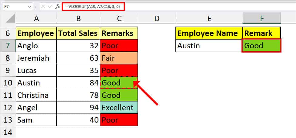
In the formula, our lookup value “Austin” is in A10. Our table range to search the item is A7:C13. Similarly, since the Remarks are in Column C, we’ve entered the 3 as Column index. By passing down a 0 boolean, the formula will return the exact match. As a result, it returned Good for Austin.
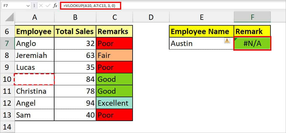
In case there was no lookup value in A10, the formula would’ve returned #N/A! Error.
Example 2: VLOOKUP with Closest Match
When you search for a value in the lookup table, it isn’t the always case you want the exact match. For number data, if you cannot find the same value in the look-up table, you would want to get the closest match instead of an error. So, in this example 2, we will use the TRUE or 1 as a range lookup argument to search for the closest match.
Example: We have a table of Product, Quantity, Unit Price, Total, Discount, and Final Total. Our Lookup Table is in J11:K14 with Amount and Discount Price.
Based on the lookup table, we want to return a discount percent for each item. As you can see the total amount is not the same. So, we will need to return the approximate value in that case.

To do this, we used the VLOOKUP formula in the box and used Flash-Fill for the rest of the cells.
=VLOOKUP(E11, $J$11:$K$14, 2, TRUE)
In the above formula, our Lookup Value is in E11 which is 1500. We will search this value in the $J$11:$K$14 table range and return the value from the second column(Discount). By passing down the TRUE argument, the formula will return either an exact match or an approximate match.
For value E11, there was an exact match. So, we got 1.5%. But, for the E12 (2556)lookup value, there isn’t the same value in the table array. So, the formula returned the closest value which is 3%.
Example 3: VLOOKUP with Partial Match
Most commonly, we tend to look for the Lookup value with the same match or an approximate match. But, the VLOOKUP function also allows you to search for the partial match of a value with the wildcard characters.
Before we start, we will first dive into the meaning of each wildcard character.
| Wildcard Character | Name | Description |
| ? | Question Mark | Select the same letter value with the same length. Example: “N?sha” will look for “Nisha,” “Nysha,” and “Nesha.” |
| * | Asterisk | Select all texts that begin or end with the specified letter. Example 1: “*e” will select values whose end letter is “e” or “E.” It could be “Title,” “Image” etc. Example 2: “e*” will count values with the initial “E” or “e” letter such as “English”, “Excel,” “eight” |
| ~ | Tilde | Select texts that contain the other two wildcard characters (? or *). Enter Tilde before a text to ensure these wildcard characters do not function as wildcards. |
Example: Suppose we have a table with First Name, Last Name, Appointment, and Service columns.

| Wildcard Character | Formula | Output | Description |
| * | =VLOOKUP(“A*”, A4:D9, 1, FALSE) | Anton | Our lookup value is (A*) in the formula. So, the formula will look for names whose initial letter is A from the table range A4:D9. Then, returns the first name with A. As a result, we got Anton. |
| ? | =VLOOKUP(“????”, A4:D9, 1, FALSE) | Lucy | Returns the name with four letters from column 1 of table A4:D9. Since the first value is “Lucy,” we got that result. But, if you had specified a letter “a” in the last like this “???a,” it would return “Anna.” |
| ~ | =VLOOKUP(“~*A”, A4:D9, 1, FALSE) | *A | The formula returned *A as it is from the first column of the table range because we use the Tilde in the beginning. If we entered just *A, it would return names that end with “a” like “Anna.” |
Example 4: VLOOKUP with Duplicate Values
From example 3, you must’ve got the gist that the VLOOKUP returns the first match from the column. Well, this is the same case for Duplicate values too. If you have a set of duplicates, you will always get the values that are on top. Besides, if it bothers you, you can remove duplicates before you use VLOOKUP.
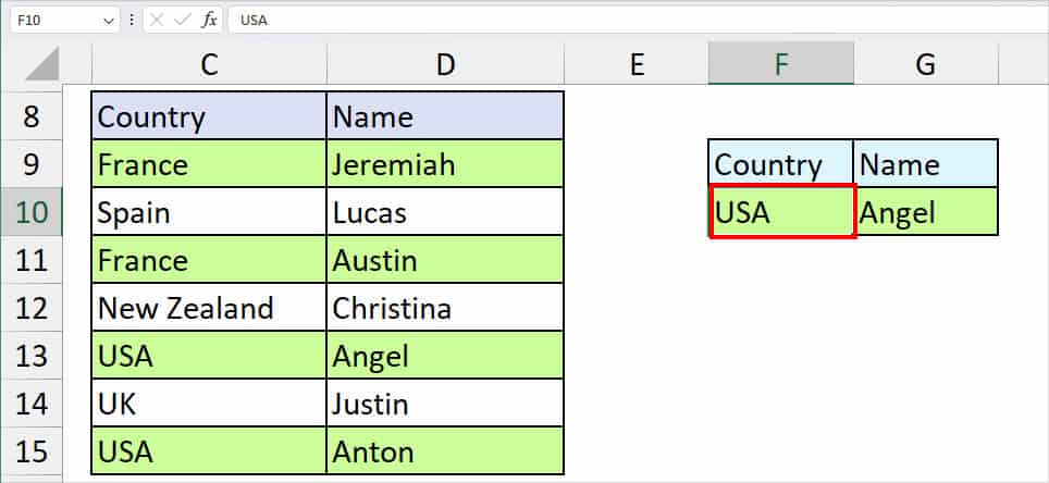
Example: I have a list of Countries and the Name of people they’re from. As you can see we have duplicates in the Country Column. Suppose, I want to look for the value of the USA.
To find this, I entered the basic VLOOKUP formula with a FALSE argument for the exact value.
=VLOOKUP(F10, C9:D15, 2, FALSE)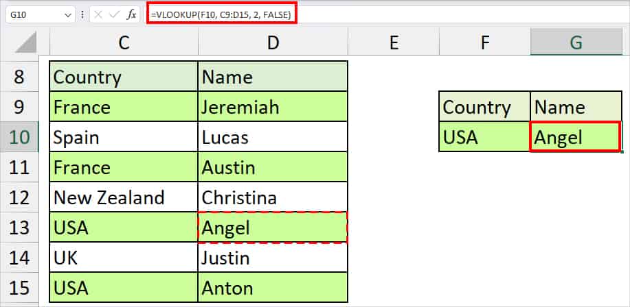
There are two USA values in the table. But, the formula returned the first name which is “Angel.”
Example 5: Merge Tables with VLOOKUP
VLOOKUP’s application is not only limited to locating the value. You could use this function to Merge two tables in Excel. But, do keep in mind that both tables must have at least one same column.
Example: Let’s assume we have two different Tables. In Table 1, we have Product, Quantity, and Unit Prices. In Table 2, we have the Product and Product ID. Since the Product column is the same, we can merge the two tables and delete Table 2.
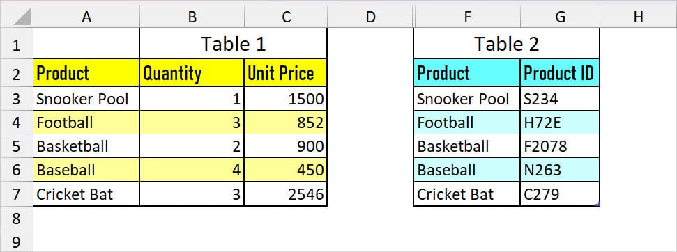
For this, I need to return the Product ID in the first table. So, I will first add a column with the Product ID and use the formula given in the box.
=VLOOKUP([@Product], Table2, 2, FALSE)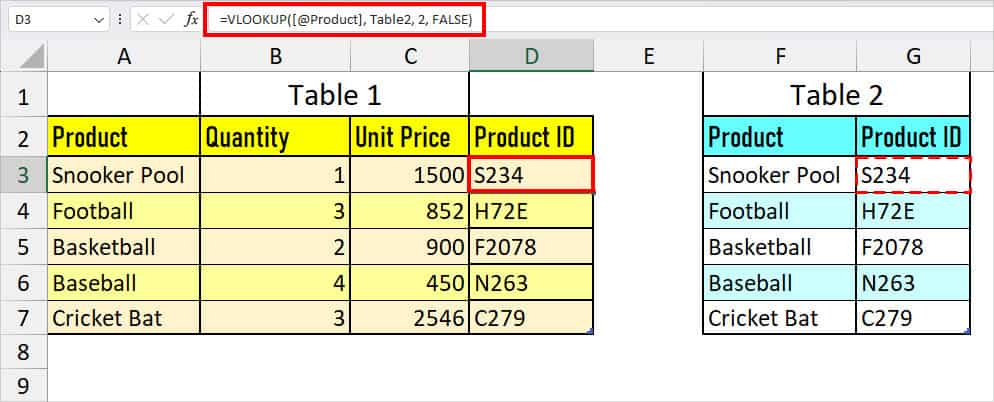
When you take a cell reference from the table in the formula, it’ll reference the value in the column header or the table name.
In our case, [@Product] is a lookup value. We’ve specified the formula to return the second column from Table 2. So, we got the Product ID in Table 1. Then, we extended the Flash-Fill handle.
Example 6: VLOOKUP with Named Range
You can use Named Ranges to shorten the VLOOKUP formula. I know the formula of the VLOOKUP function solely isn’t long. But, it could get lengthy when you nest the function with others. Entering a Named Range in VLOOKUP is somewhat similar to a Table Reference.
Example: Suppose we have named the lookup table A7:C13 as Employee. Let’s return the remark of Lucas in cell F8.
For this, our formula will be
=VLOOKUP(E8, Employee,3,FALSE)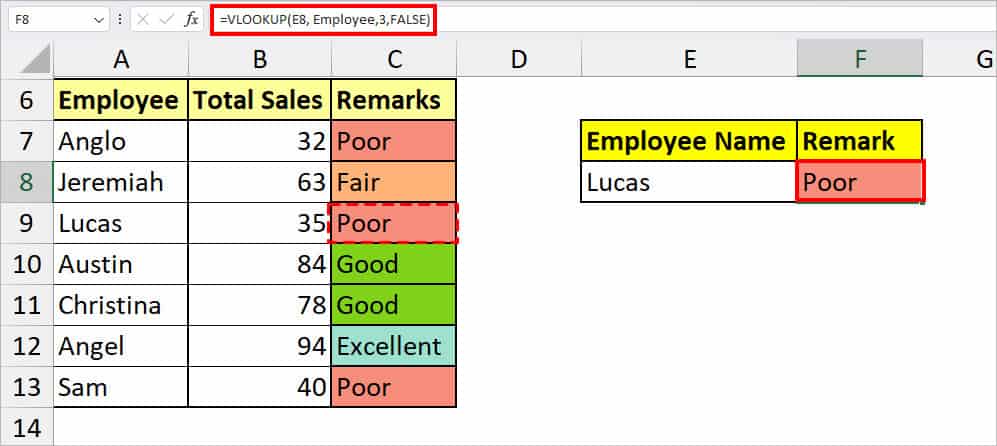
Here, the lookup value (Lucas) is in E8 and our Table range A7:C13 is Employee. We’ve specified the formula to return the exact value from the third column. As a result, we got Poor.
Example 7: Use VLOOKUP Across Different Sheets
If we take a closer look into the practical scenario, VLOOKUPs are mostly used to draw out the data from different sheets than in the same sheet. So, now that you have learned all 6 cases of VLOOKUP within the same sheet, we will move on with the separate sheets.
For any formula that involves sheet references, it’s important you know the basic rules of the Sheet Reference first. You can check out our other article where we’ve discussed all types of references between a sheet with examples.
Here’s the formula to use the VLOOKUP function across different sheets.
=VLOOKUP(lookup_value, SheetName!table_array, col_index_num, [range_lookup])Example: Suppose, we want to pull the data of the Product ID column from ProductSheet to our MainSheet.
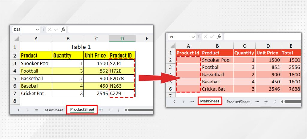
To do this, we entered this formula
=VLOOKUP(B2, ProductSheet!A3:D7, 4, FALSE)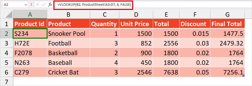
In formula B2 (Snooker Pool) is our look-up value from MainSheet. Our table array is A3:D7 table range of ProductSheet. Since we’ve passed down fourth column, the formula will return the Product ID. We got S234 in the formula cell and dragged down the fill handle for other cells.
Although you can type a formula, we’ll teach you an even simpler way to input the formula.
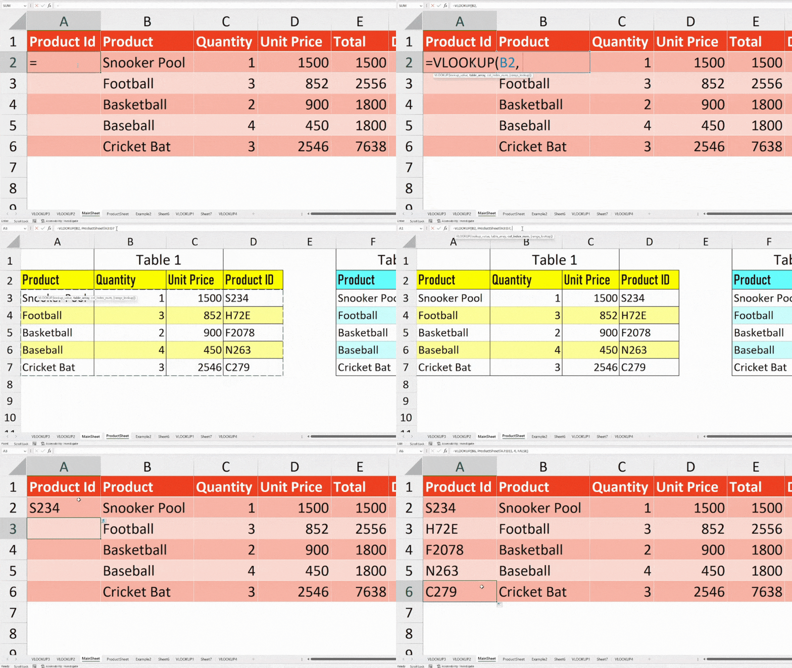
- Firstly, enter =VLOOKUP(
- Select the Cell that contains the lookup value and enter a Comma.
- Go to Another sheet and select the Table range, (,), type Column Index, (,), TRUE or FALSE. Close the bracket and press Enter.
Example 8: Use VLOOKUP in Different Workbooks
Just like how you can pull out data from a separate sheet in Excel, it is also possible to extract items from different workbooks. But, of course, you need to keep both workbooks open before you enter the formula.
Formula: VLOOKUP(lookup_value, [Workbook.xlx]SheetName!table_array, col_index_num, [range_lookup])Example: Suppose my co-worker has a list of Students’ names, Groups, and Science scores in her workbook. But, in my sheet, the Group name is missing. So, let’s get the Group Name from the Worbook named “Student Score.”
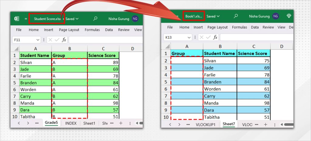
To do so, I used the following formula
=VLOOKUP(B2, '[Student Score.xlsx]Grade5'!$A$2:$C$11, 2, FALSE)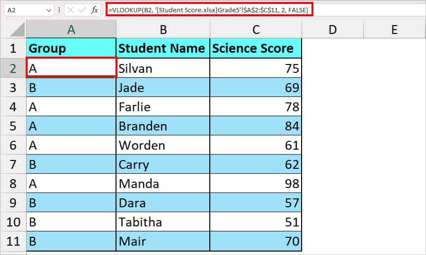
The VLOOKUP function returned the Group name from the Student Score Workbook, Grade 5 Sheet, $A$2:$C$11 table range, and second column.
Here’s how we entered the formula.
- Firstly, enter =VLOOKUP( and select a cell with Lookup_value. Enter Comma.
- Now, navigate to Another workbook and select the Table range, (,), enter Column index, (,) TRUE or FALSE. Close the Bracket and press Enter.
How to Make VLOOKUP Function More Dynamic?
When you reference a cell or value in the VLOOKUP function, you’ll get result only for that specified item. In that case, you would have to change the arguments for lookup value every time to search for another item. But, Hold on!
There’s a way to make your VLOOKUP function dynamic. We can create a drop-down list for the lookup value cell and switch items. When you do this, the formula would automatically update formula according to the lookup value. So, why not use this feature in your favor?
- Click on the Lookup value cell. Let’s say our cell is F10.
- From Data Tab, click Data Validation in the Data Tools section.

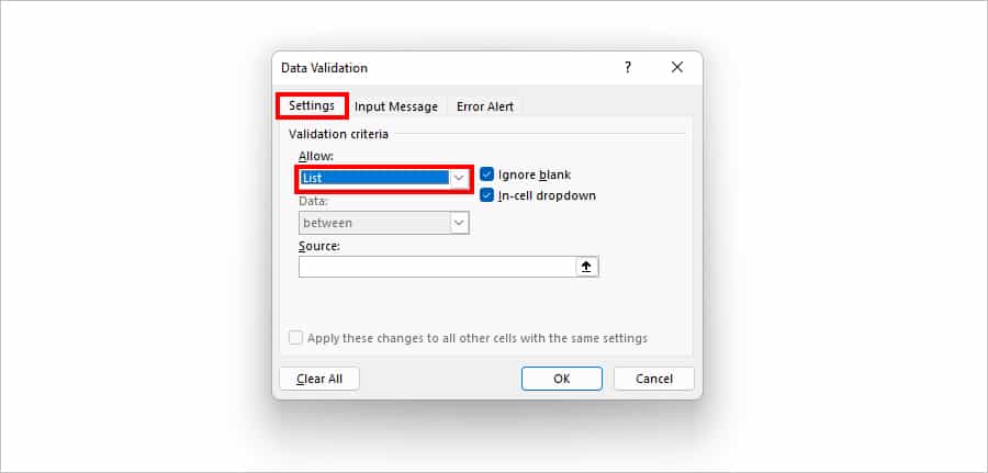
- On the Data Validation dialogue box, stay on the Settings tab. Then, below Allow, choose List.
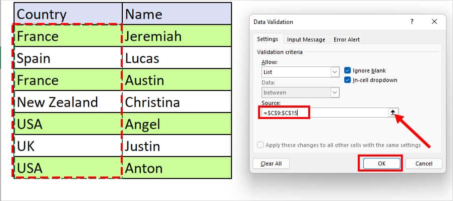
- On the Source menu, use the Collapse icon and select the array of lookup values from the lookup table. Click OK.
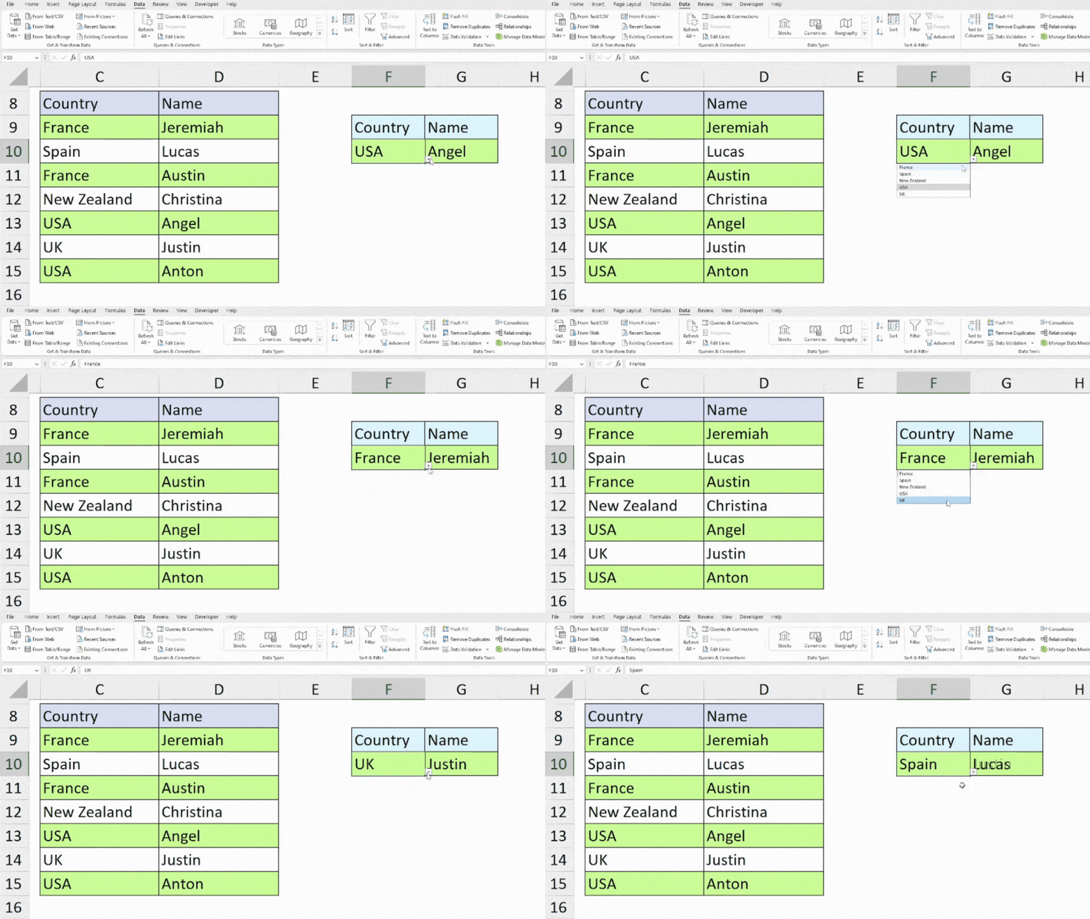
- Now, when I switch the lookup value, the VLOOKUP formula will auto-update.
Avoid Errors When Using the VLOOKUP Function
When using the VLOOKUP function, you may get these cell errors in the formula. But, if you know the causes that result in the error beforehand, it is possible to avoid them.
| Error | Possible Causes |
| #N/A Error | Look up value not found. Incorrect Column Index. The formula cannot look to the left of the lookup column. |
| #NAME? Error | Spelling Error in Texts Arguments. Not Double Quoting (“”) Text Arguments. |
| #VALUE! Error | When Table_array > 1. |
| #SPILL! Error | When you pass down an entire column as a lookup value. |
| #REF! Error | If the Column Index number in the formula is more than the columns of table_array. |
| #FILED! Error | When there’s a full stop (.) instead of comma (,) in the formula. |
| Incorrect Result | When the values are not sorted in alphabetical or numerical order while using the TRUE argument. When numbers or dates are in text format. |
Alternative to VLOOKUP Function
| Function | Syntax | Description |
| XLOOKUP Function | =XLOOKUP(lookup_value, lookup_array, return_array, [if_not_found], [match_mode], [search_mode] | Searches lookup_value in the specified lookup array and extract the value from a return array. Try the XLOOKUP function when you want to draw out an array of lookup values in both vertical and horizontal arrays. It also supports multiple criteria. |
| INDEX and MATCH Function | =INDEX(array(MATCH(lookup_value, lookup_array, [match_type]) | With INDEX and MATCH functions nested together, the formula returns lookup_value from any column index. You could use this function when the Lookup Value isn’t in Column 1. |
Author’s Note: We’ve discussed everything about using the VLOOKUP Function with the single criteria in this article. If you want to learn How to Use VLOOKUP with Multiple Criteria from scratch, check out this detailed guide.