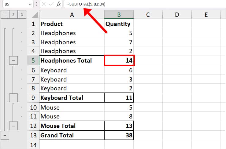
Excel’s SUBTOTAL function is the formula version of the Subtotal feature. It is one of the Math and trigonometry functions used to calculate the subtotal of the items.
The specialty of the SUBTOTAL function is that it works with other functions like AVERAGE, PRODUCT, SUM, COUNTA, and many more to return the amount based on criteria. For example, you could calculate the product of the subtotal in a given range or count the subtotal.
Arguments for SUBTOTAL Function in Excel
As the name itself says, the SUBTOTAL function returns the subtotal in a given database.
Syntax: SUBTOTAL(function_num, ref1, [ref2],...)The SUBTOTAL function takes up the function number and cell references as arguments.
- function_num: Function number to specify the SUBTOTAL to use it. Eg: 1, 9, 110, etc.
- 1-11: Takes Hidden rows
- 101-111: Avoids Hidden Rows
- ref1: Cell ranges or Named ranges to calculate the subtotal.
- [ref2]: Additional cell ranges to return the subtotal from
Remember, the arguments inside the () parentheses are required while the ones with [] parentheses are optional.
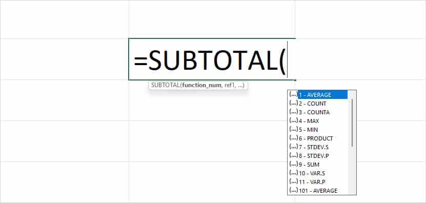
In the given table, we have compiled the function name and description of each function_num to make it easier for you to enter the argument. However, you do not have to remember or note all of this down. When you start typing =SUBTOTAL( formula in the cell, it displays a drop-down list for the function_num. You can simply choose one.
So, now, let’s see what 1-11 and 101-111 mean in the function_num.
| Function Name | Function Description | (function_num: 1-11) Takes Hidden rows | (function_num: 101-111) Avoids Hidden rows |
| AVERAGE | Returns arithmetic mean from the number data. | 1 | 101 |
| COUNT | Counts and returns the total number of cells that has a numerical value. | 2 | 102 |
| COUNTA | Counts and returns the total number of nonempty cells. | 3 | 103 |
| MAX | Returns the highest or largest number from cell ranges. | 4 | 104 |
| MIN | Returns the lowest or smallest number from cell ranges. | 5 | 105 |
| PRODUCT | Returns the product between the given numbers or cell ranges. | 6 | 106 |
| STDEV | Calculates the Standard Deviation from the specified sample. | 7 | 107 |
| STDEVP | Returns the Standard Deviation of the Population. | 8 | 108 |
| SUM | Calculates the total sum of numbers. | 9 | 109 |
| VAR | Estimates and returns the Variance of a given sample. | 10 | 110 |
| VARP | Returns the variation of a population. | 11 | 111 |
Things You Should Know Before Using the SUBTOTAL Function
- The SUBTOTAL function ignores the existing SUBTOTAL function. For Example, let’s assume you’ve used the SUBTOTAL formula in cell B6. If you enter cell B3:B10 in a formula, it bypasses the value of B6.
- Whether you pass down the 1-11 or 101-111 function argument, the SUBTOTAL function discards the filtered value. But, if you choose to display the filtered items later, the function will automatically include them again.
- 1-11 or 101-111 function argument rule applies for rows only. Meaning, the rule is invalid for Columns. For example, if Column B is hidden, the SUBTOTAL function includes the value of Column B too. So, even if you enter =SUBTOTAL(102, B5:D5) or SUBTOTAL(2, B5:D5), the result will be the same.
- The SUBTOTAL function ignores Text strings in a cell value while using some functions like PRODUCT, COUNT, SUM, etc
- You cannot enter function numbers except for 1-11 or 101-111. If you do, Excel will send you a #VALUE! Error.
Examples of Using the SUBTOTAL Function
Below, we have covered five examples of using the SUBTOTAL function. We have discussed about hidden, non-hidden, and filtered rows in the data.
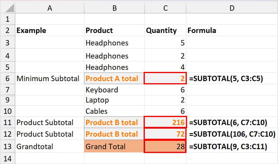
| Example | Formula | Result | Description |
| Minimum Subtotal | =SUBTOTAL(5, C3:C5) | 2 | Calculates the lowest subtotal value. |
| Product Subtotal | =SUBTOTAL(6, C7:C10) | 216 | Returns the product subtotal from the cell range C7 through C10. As you can see in the picture, cell C8 is hidden. Since we passed down 6 as function_num in the formula, it also takes in the value of C8. |
| Product Subtotal | =SUBTOTAL(106, C7:C10) | 72 | Multiplies the numbers in cell range C7 through C10. Again, here, cell C8 is manually hidden. But this, time the function_num (106) won’t include the hidden cell. So, we got a different answer. |
| Grand Total | =SUBTOTAL(9, C3:C11) | 28 | Calculates the sum of cell ranges from C3 through C11 including the hidden cell. Since we have a SUBTOTAL formula in cells C6 and C11, it ignores these cells when returning the total. |
| Grand Total | =SUBTOTAL(9, C3:C11) | 19 | Calculates the sum of cell ranges from C3 through C11 including the hidden cell. This time we got a different result because we filtered some items from the Product column. So, even though we entered function_num (9), it discarded the filtered values. |
Common Errors to Avoid When Using SUBTOTAL Function
When using the SUBTOTAL function, #VALUE! error may arise if there is an error in the function_num argument. It could also occur if you’ve entered a 3-D reference in the cell ranges.
Similarly, if there’s a typo in the formula name itself, it’ll return #NAME? Error. With that said, you will get #DIV/0! Error when the function_num you’ve used in the formula is dividing by 0. So, be careful and make sure to use the correct arguments in the formula to avoid errors.
An Alternative of SUBTOTAL Function
Excel also has a SUBTOTAL menu in the Data tab which works similar to the SUBTOTAL function. Here, you just need to enter the information in the Subtotal window. Excel will construct the formula for you. If needed, you can also edit the formula from the formula bar.
Note that to use this feature, data in cell ranges after each Column header must be the same. Before you begin, make sure to sort the Column in A to Z or Z to A order. Here’s an example in the picture.
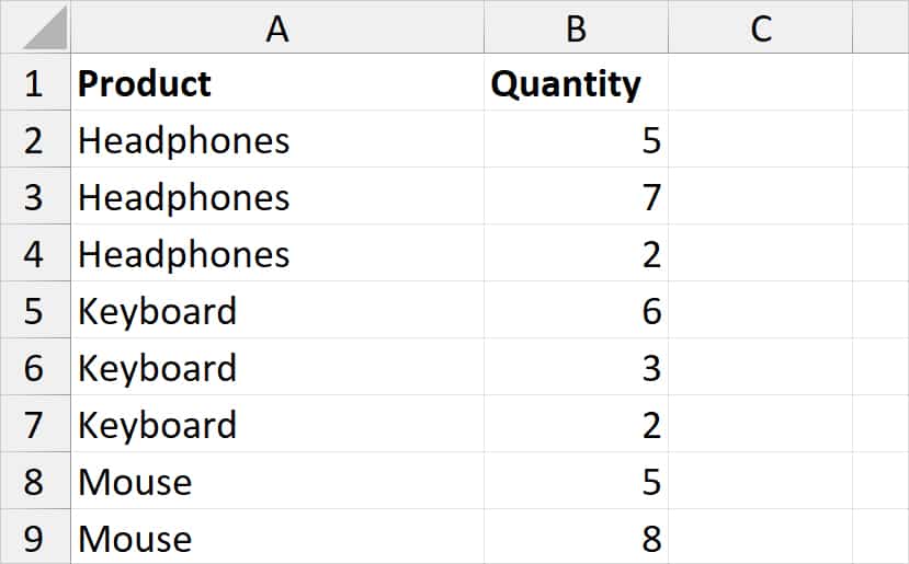
- On your sheet, select all data.
- Head to Data tab and click on Subtotal menu in the Outline group.

- On the Subtotal window, do the following:
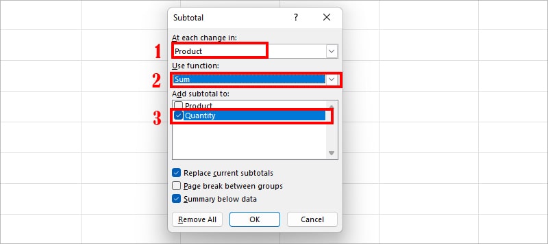
- At each change in: Choose a Column Header
- Use function: Pick the Function to use in Subtotal
- Add subtotal to: Select Columns to return the Subtotal result in
- Leave the options with the checkboxes as it is and click OK.
- You’ll get the Subtotal for each product. If you click on the output, you can also see the result in the formula bar.
