When arranging full names in Excel, you may find the need to reorder them by Last Name, especially when you have to emphasize the Family Name.
But, while sorting data, Excel always takes the first word or text string as a sort order. So, when you have a Full Name, it means that the names are alphabetized by First Name.
However, we have 5 easiest workarounds to help you reorder by Last Name.
Using Flash Fill
If you enjoy Excel’s Flash Fill, I have good news as you can use it to rearrange data by Last Name. But, it’s best only when you have a few names.
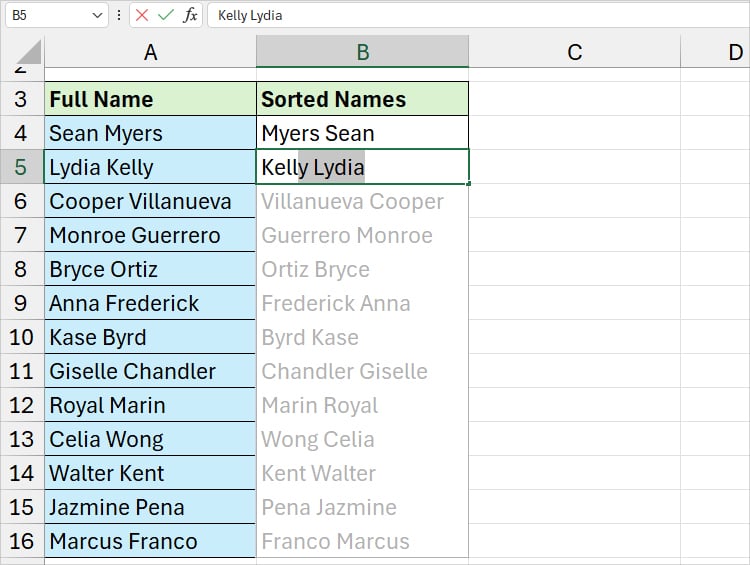
In the next column, type the Names in Last, First order and press Enter. The Flash-fill will automatically suggest you fill the cells in the same pattern.
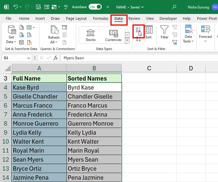
Once you have entire names, go to the Data Tab. Click on the A to Z menu. You will have data sorted by last name.
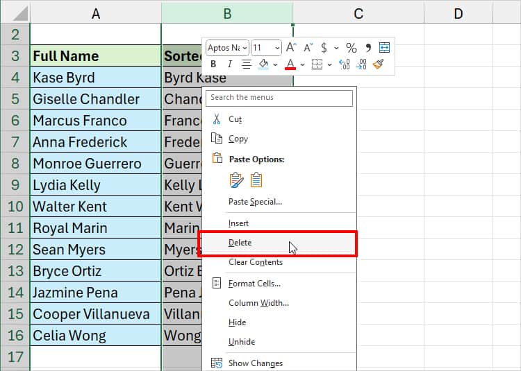
Selected the Sorted column. Right-click on it and click Delete.
As I mentioned earlier, this approach is best for only a small dataset as it could be redundant over time and bore users.
Using Find And Replace
Another way to sort by family name is using the Find and Replace tool. Here, we will insert a new helper column with last names only.
Then, set it as Sort by in the Sort window. You can delete that extra column once you’re done.
- First, copy-paste the Names into your Adjacent Column.
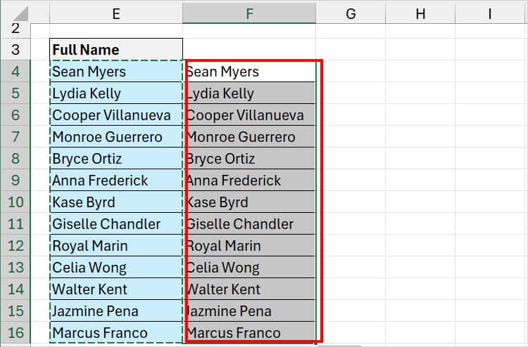
- Now, select your Names. Then, press
Ctrl + HFind and Replace Menu Shortcut. - On Find What, type the Asterisk sign and Space key.
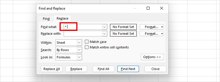
- On Replace with, leave the field empty and click Replace All. Now, you will only see Last Names in the Column.
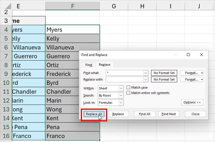
- Select All Data. From the Data tab, click the Sort button.

- On Sort by, choose Last Name. On Order, choose A to Z or Z to A and click OK.
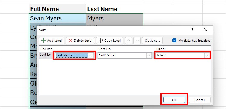
- Finally, you can delete the Last Name column.
Using Text to Columns
The Find and Replace is useful when your Names have space in between them.
But, Let’s say your Names are separated with a comma or dash delimiters. If that’s the case, you could opt for Excel’s Text to Columns Wizard to split columns and then reorder the names by last name.
- Firstly, select the Ranges with Names.
- On the Data Tab, click Text to Columns.

- In Step 1, hit Next.
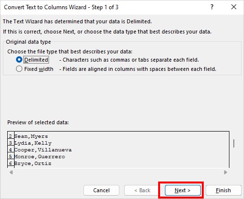
- On Step 2, tick any one Delimiters option. If you don’t see your Delimiter, tick Other and type the sign. Choose Next.
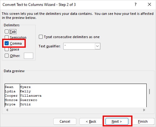
- While the First Name is selected, choose Do not import column. Select Cell range in Destination and hit Finish.
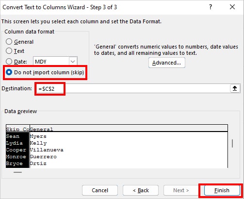
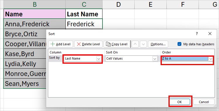
- Now, select all. On Data, click Sort. On Sort By, select the Last Name Column. Pick your Sort Order, and click OK.
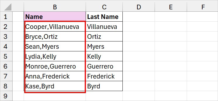
- Here are the Sorted Names. Delete the Last Name if you want.
Using Power Query
If you don’t want to copy-paste, add new columns, etc in your sheet, I have more simpler way of sorting the data.
This time we will load the Names into the Power Query Editor tool and perform everything there that takes only a few clicks.
- Select your data.
- In the Data Tab, click on From Table/Range. Choose OK on the prompt.

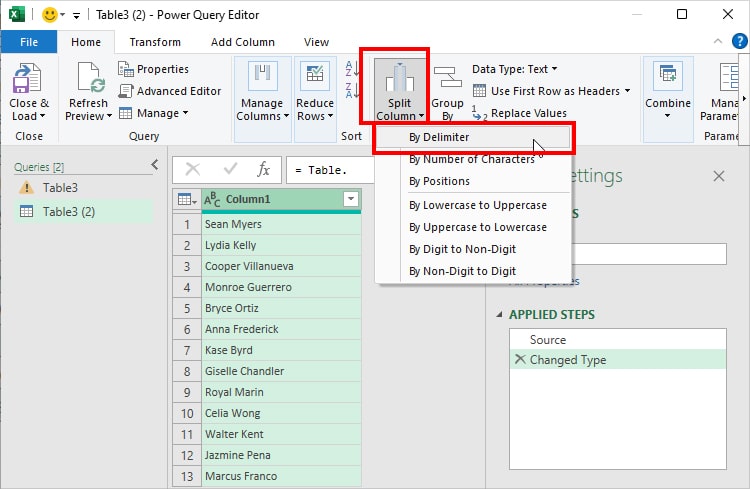
- Now, on the Power Query Editor tool, select the Names Column. In-Home Tab, click Split Column > By Delimiter.
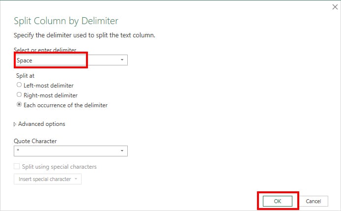
- On the Split Column by Delimiter window, select delimiter and hit OK.
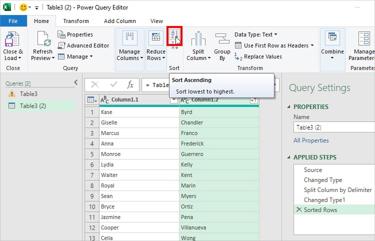
- Now, select the Last Name Column and click Sort Option in the Home tab.
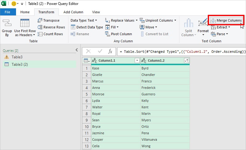
- Finally, to merge the names again, select both columns. Go to the Transform tab and click on Merge Columns.
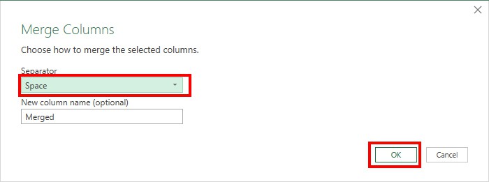
- On Merge Columns, pick Separator and click OK.
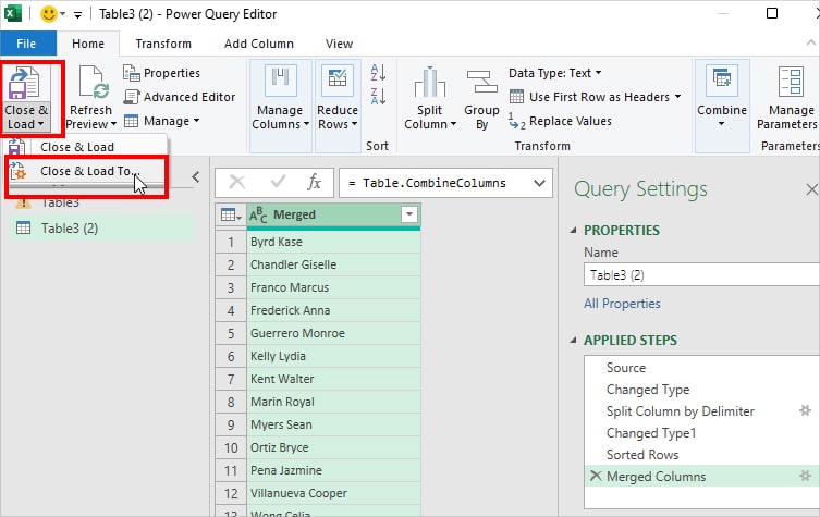
- Select the Merged Column. Head back to the Home Tab and click Close & Load > Close & Load To.
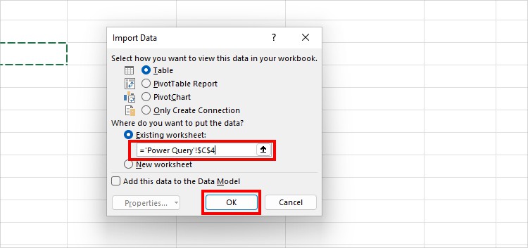
- On Import Data, choose Location to load data and hit OK.
Using Formula
Next, you could also split and merge columns using the Formula in Excel. However, to reorder the data, we will use the same Sort button.
Although the steps are long, it’s more dynamic than the rest of the methods mentioned above.
Suppose, I have a list of Full Names in Column D. I will enter each formula to extract the First and Last Names separately in Column F and G respectively.
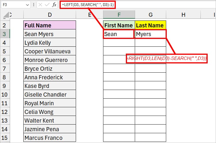
| Extract | Formula | Description |
| First Name | =LEFT(D3, SEARCH(” “, D3)-1) | Using the SEARCH and LEFT nested formula, we will return the text before the space in D3 from the left side. We got Sean as a Result. |
| Last Name | =RIGHT(D3,LEN(D3)-SEARCH(” “,D3)) | Here, we have specified the formula to return the texts from the right after the space. It resulted in Myers. |
Then, extend the Fill Handle.
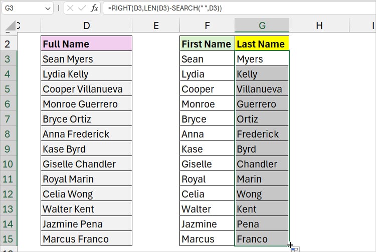
Now, using the Ampersand Operator, we will combine the Names in the Last, First order separated by a comma. After that use the Auto-Fill to fill in the remaining cells.
Formula:
=G3&", " &F3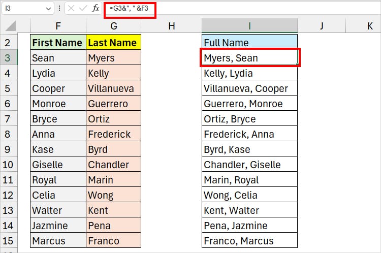
Copy-paste the Column as Values Only. Now, select the Column Range. Right-click on Column > Sort. In the Context menu, click A to Z or Z to A. It’ll sort your column by Last Name.
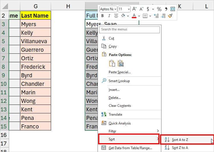
Lastly, you can separate the sorted Names with Text to Columns.
After that, use Concat to combine those names as First Name, Last Name.