You can find users calculating Growth Rates for every aspect or industry. For Instance, Economists calculate the Growth rate to assess GDP (Gross Domestic Product), Businesses to find out the company’s investment return, biologists to study the population size, etc.
However, in Excel, mostly financial analysts or business managers tend to evaluate the Growth Rate for the company’s decision-making. So, we will be guiding you on how to calculate the Growth Rate with a simple example of Sales and Revenue in this article.
Growth Rate – Overview
If there’s a percentage change in the value over a certain period of time, it’s called a Growth Rate. A growth rate can be Positive or Negative.
If the value has risen over time, it’s a positive growth. Similarly, when the variable has been declining over time, it indicates a Negative growth. Normally, Growth Rates are calculated Annually, Quarterly, Monthly, or Weekly time period.
The formula to calculate the Growth Rate is pretty simple. We will be using the same formula in Excel too.
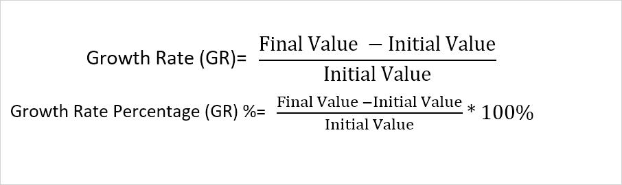
Formula: = Final Value - Initial Value/Initial ValueExample: Here, I have a Chocolate Chip Cookies Sales list for 2022 and 2023. Let’s calculate the Growth Rate of a year using the formula.
In the Growth rate column, I entered the formula as
=(C2-B2)/B2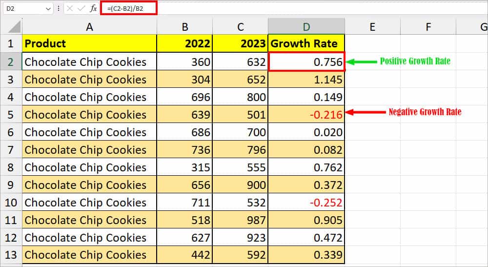
In the formula, C2 is my Final Value and B2 is my Initial Value. The formula returned 0.756. Once you get the result, drag down the formula to other cells using Auto-Fill.
Here, the numbers with a minus sign show the negative growth rate. You can even apply a cell style or conditional formatting to highlight that negative number.
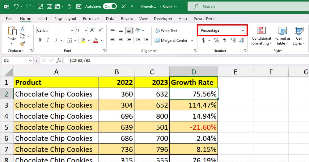
In case, you want the percentage, change the formatting to Percentage from the Home Tab.
Average Annual Growth Rate
The Average Annual Growth Rate measures the average return on investment over time. Here, we will calculate the arithmetic mean of growth rates.
The formula for the Average Annual Growth Rate is
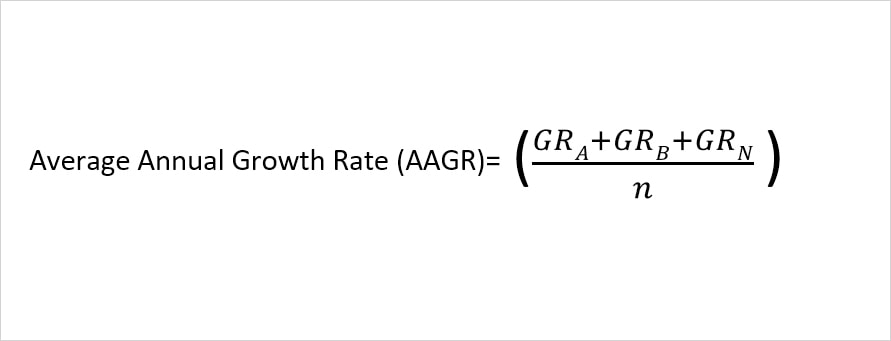
=(GRA + GRB + GRn)/ nHere,
- GRA: Growth Rate in Period A
- GRB: Growth Rate in Period B
- GRn: Growth Rate in Period n
- N (n): Number of payments
But, to find out the Average Annual Growth Rate, we won’t be using this formula in Excel like the Growth Rate. Instead, we will use the AVERAGE function to return the average value of the Growth Rate.
This means there are two steps you need to follow. Firstly, you must calculate the Growth Rate and then the Average value.
As an example, we will take the same example as above. Suppose, I have already calculated the Growth rate and it lies in Columns D2 through D13. Now, we will use the AVERAGE function to calculate this.
=AVERAGE(D2:D13)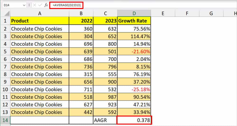
The Average Function returns the arithmetic mean from the specified range. Here, I got 0.378 as a result. After you get the results, you could also convert the number into the percentage format.
Compound Annual Growth Rate
The Compound Annual Growth Rate (CAGR) measures the yearly growth rate of an investment over a duration. The formula to calculate the Compound Annual Growth Rate is:
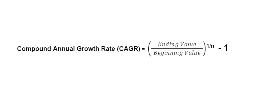
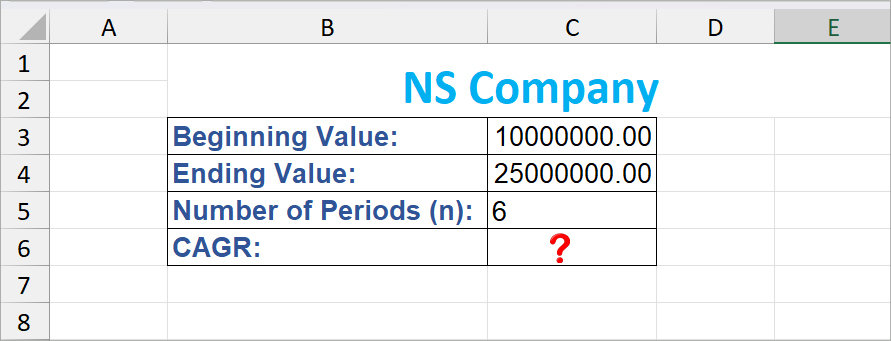
=(Ending Value/Beginning Value)1/n - 1Example: Let’s assume the NS company has a revenue of $10 million at the end of the current period (Year 0). The company’s revenue is projected to be $25 million in the six years from the present date (Year 6). Let’s find out the CAGR for NS company.
From the example, we will first input each component of the formula to calculate them.
Here,
- Beginning Value (C3): $10 million
- Ending Value (C4): $25 million
- Number of Periods (n) (C5): 6
To calculate the CAGR, we used the same formula as above which is
=(C4/C3)^(1/C5)-1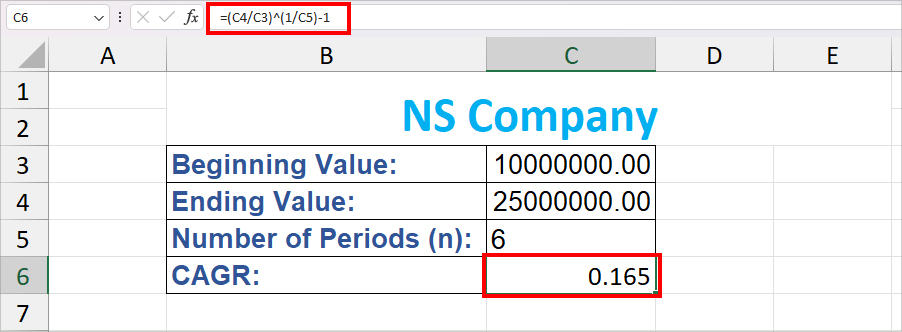
The formula returned a 0.165 CAGR value. Here, we’ve used the cell references such that the formula auto-updates whenever you edit the value in the cell. You can enter the number too.
Also, you may have noticed we used the caret sign to enter the 1/n power for the formula. It’s a lot easier to reference the value as a power number using that sign.