How to Build Games in Excel (With or Without VBA)

You can run some really cool games in Excel, but did you know you could build one yourself? 

While Macros are mostly used in automating tasks in Excel, they can also be used to build games. If you’re familiar with the Visual Basics for Application (VBA) code, then you can use this language to build your own game from scratch.

Even if you are new to coding, don’t worry! We have created a step-by-step guide to build some of the most popular games in Excel without using the VBA code.

Build Games Using the VBA Code

Excel uses the Visual Basics for Application code to create functions and record macros. You can build a macro to run a game of your choice using the VBA code.

You will have to create a macro for your game, enter its code, and then run it. You can create and use a Macro from the Developer tab. The Developer tab is disabled on Excel by default, so you will have to enable it from the Excel Options. Once you enable the utility, follow these steps to build a game using VBA.

Step 1: Create a Macro

1. Head to the Developer tab.
2. Select Macros from the Code section.
   
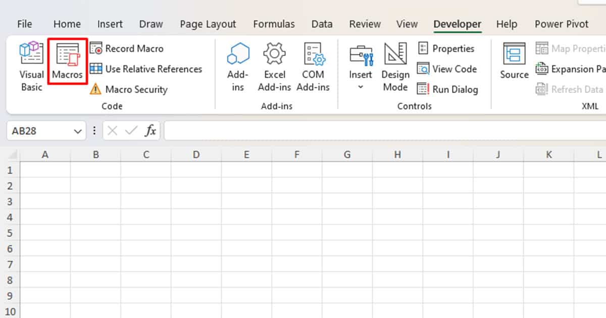
3. Enter a name for your macro and click Create.
   
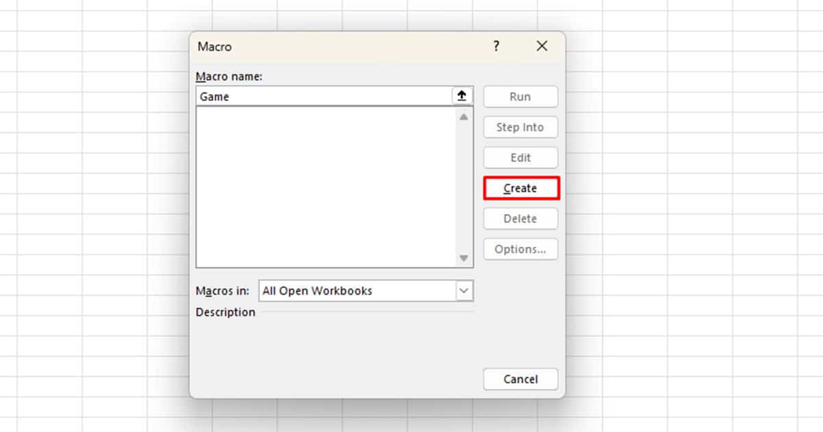
4. On the Visual Basic Editor window, enter the code for your game.

Step 2: Run your Macro

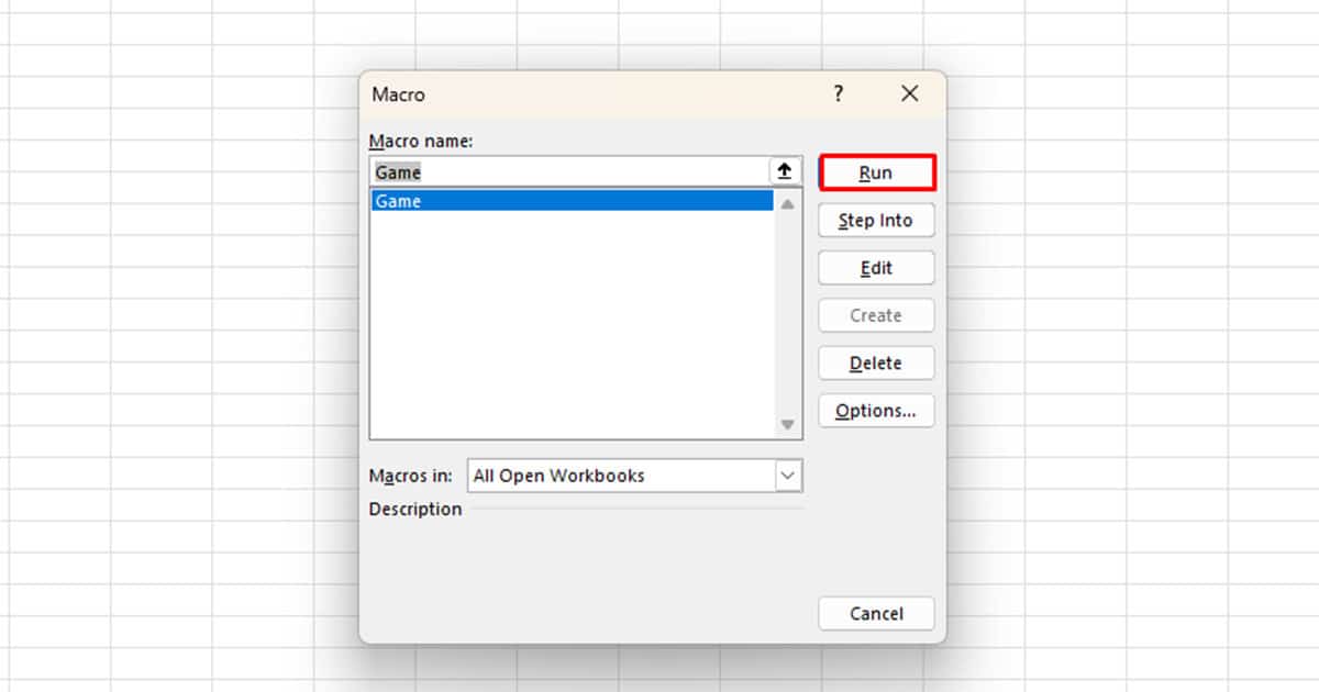
1. Go to Developer and select Macros from the Code section.
2. Select your macro from the list.
3. Click Run.
   

Build Games without Using VBA

Excel has enough tools and features to help you create a game. While you can get creative with the abundant Excel features, we have arranged four games you can build without using the VBA code. These games include Poker, Snakes and Ladders, Trivia, and TicTacToe.

Slot Machine

The slot or poker machine is one of the few games that really gets the crowd to go berserk. This is completely based on luck where each player has the chance of getting three identical numbers or symbols.

We can use the RANDBETWEEN function in Excel to create a similar interface on our spreadsheet. A typical slot machine has about 20 symbols in each reel. Therefore, we can construct our RANDBETWEEN function in this formula:

=RANDBETWEEN(1,20)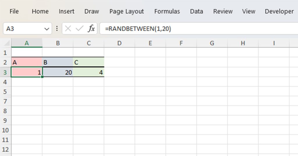

Copy-paste this formula into three adjacent cells. To refresh the values, hit the F9 key on your keyboard. We can also use the IF function to create a confirmation message for if you’ve won or lost using this formula:

=IF(A3=B3=C3, "YOU WON!","TRY AGAIN!")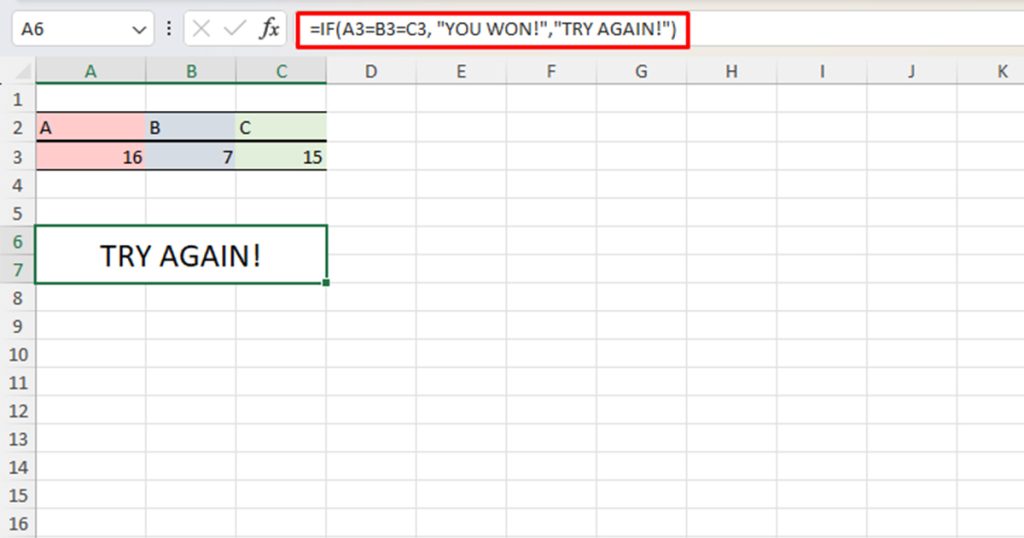

You can then use Excel’s formatting tools, and merge cells to decorate your sheet to give it that arcade-like feel.

TicTacToe

Excel’s grid interface makes it amazing to play a game of TicTacToe. While you can start drawing knots and crosses on the sheet as it is, there are a few formats you can tweak to make it perfect for playing tic-tac-toe.

Step 1: Resize the Cell

The default row and column size of a cell in Excel is 15 and 8.43 respectively. This dimension isn’t as visually appealing when playing a game of TicTacToe. As a workaround, we can resize the cells to fit our texts.

1. Select nine adjacent cells from your grid.
2. On the Home tab, select Format from the Cells section.
   
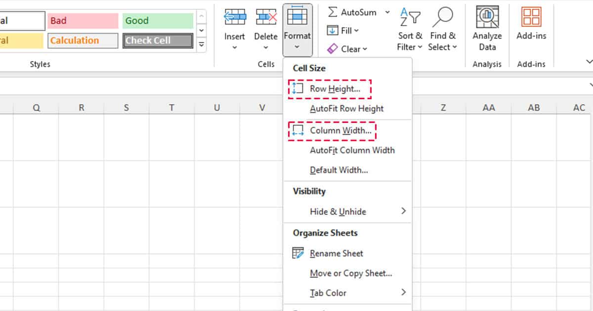
3. Click on Row Height and change the value to 50.
   
4. Click OK.
5. Using step 2, click Column Height and enter 10.
   
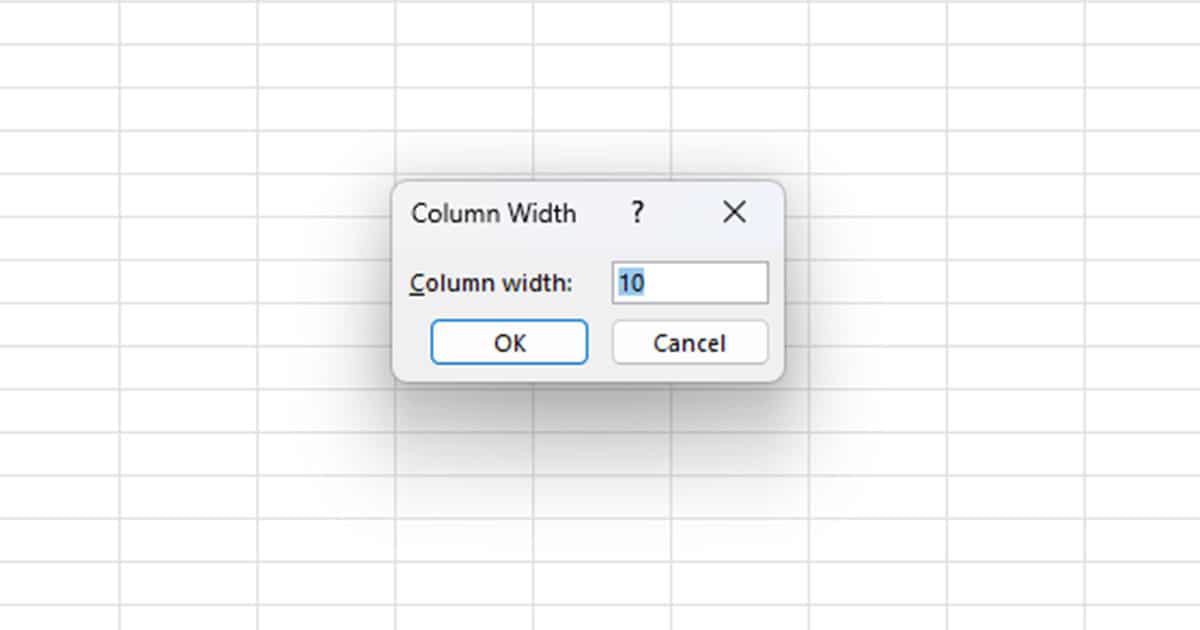
6. Click OK.

Step 2: Add Borders

After resizing your cells, you can add borders to the cells to distinctly partition them from each other. You can apply the Right borders on the first two columns. Then, apply both the Top and Bottom borders to the middle row of the TicTacToe grid.

Here’s how we applied borders on our grid:

1. Select range A1:A3.
2. Go to Home and from the Font section, click the fly-out for borders.
3. Choose the Right border.
   
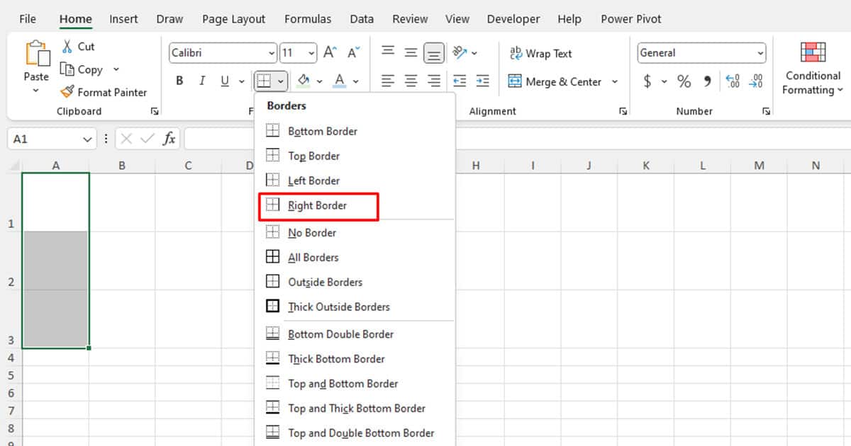
4. Select range B1:B3 and repeat steps 2 and 3.
5. Select range A2:C2 and head to the borders menu.
   
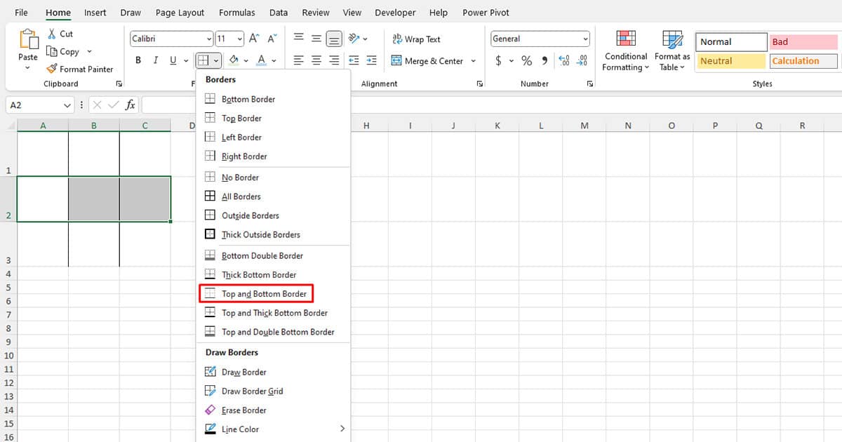
6. Choose the Top and Bottom border.

Step 3: Change Font Size and Alignment

By default, Excel uses the font size 11, and left alignment for text values. It goes without saying that this format is not ideal when it comes to a game of TicTacToe.

Let’s change the font size to make our texts appear bigger, and the alignment to keep our text centered.

1. Select your range.
2. On the Home tab, select the fly-out for the font size and choose 48.
   
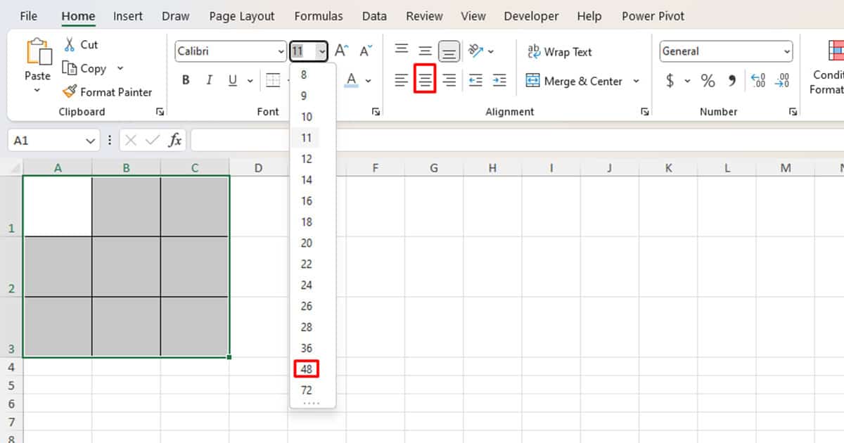
3. From the Alignment section, click on the Center alignment.

Step 4: Start Playing!

Voila! Here’s the perfect interface for you to play TicTacToe with your peers. If you feel the gridlines are a distraction, you can head to the View tab and uncheck the box next to Gridlines. Enjoy your game!

Quiz

You can create a multiple-choice Quiz in Excel using Data Validation. You can also use this format to host trivia nights with your buddies.

To make the quiz look more appealing, we can also use Conditional Formatting to shade cells that are correct as green and the incorrect ones as red.

Step 1: Enter Questions

Take, for instance, you have six questions. You can enter your question on the top cell and create a drop-down list at the bottom for the answers.

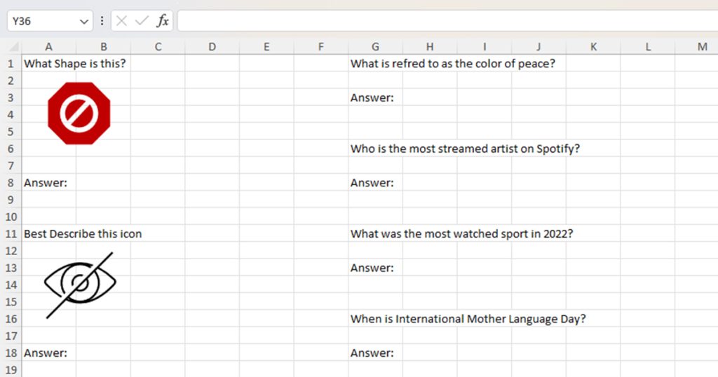
Step 2: Create Multiple Choice Answers

To create a drop-down list on a cell, follow these steps:

1. Select the cell you wish to insert the drop-down list.
2. Head to the Data tab.
3. From Data Tools, select Data Validation.
   
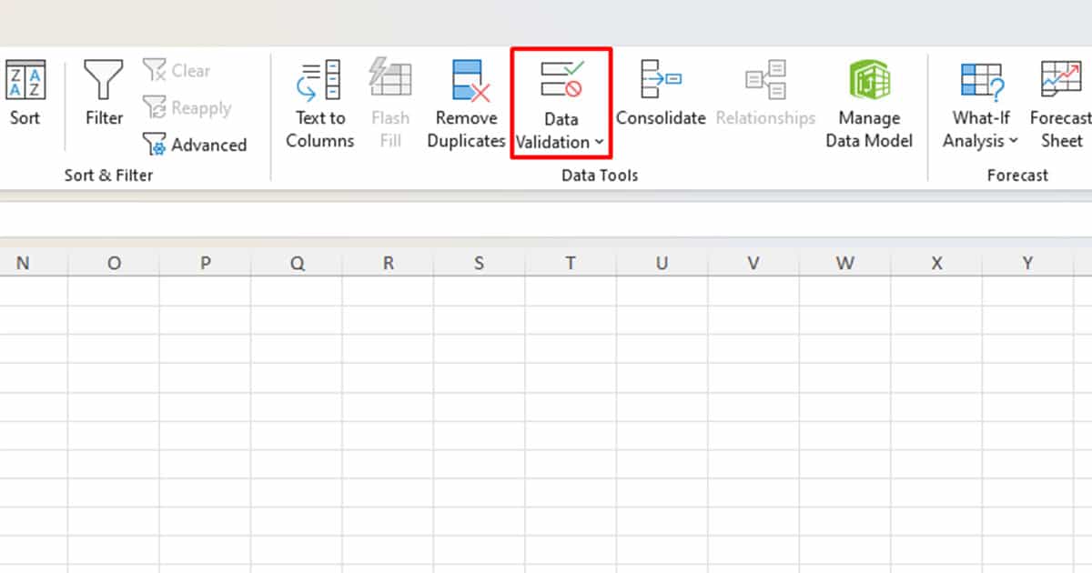
4. Under Allow, choose List.
5. Under Data, enter the answer choices separated by a comma.
   
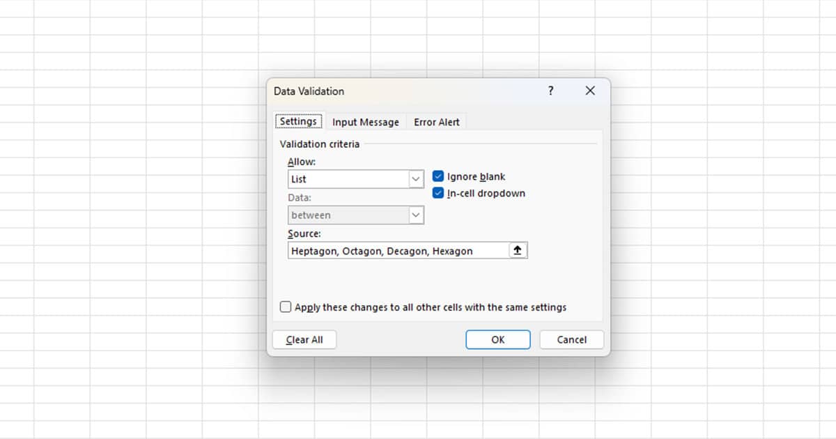
6. Click OK.

Step 3: Apply Conditional Formatting

To Format Correct Answers:

1. Select the cell with answers.
2. Go to Home and choose Conditional Formatting from the Styles section.
3. Choose Highlight Cells rules > Equal To
   
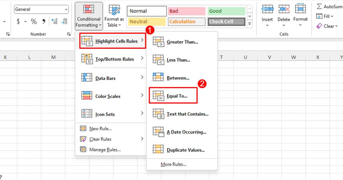
4. Enter the correct answer and choose the appropriate formatting on the next option.
5. Click OK.

To Format Incorrect Answer:

1. Go to Home and select Conditional Formatting.
2. Select New Rule.
   
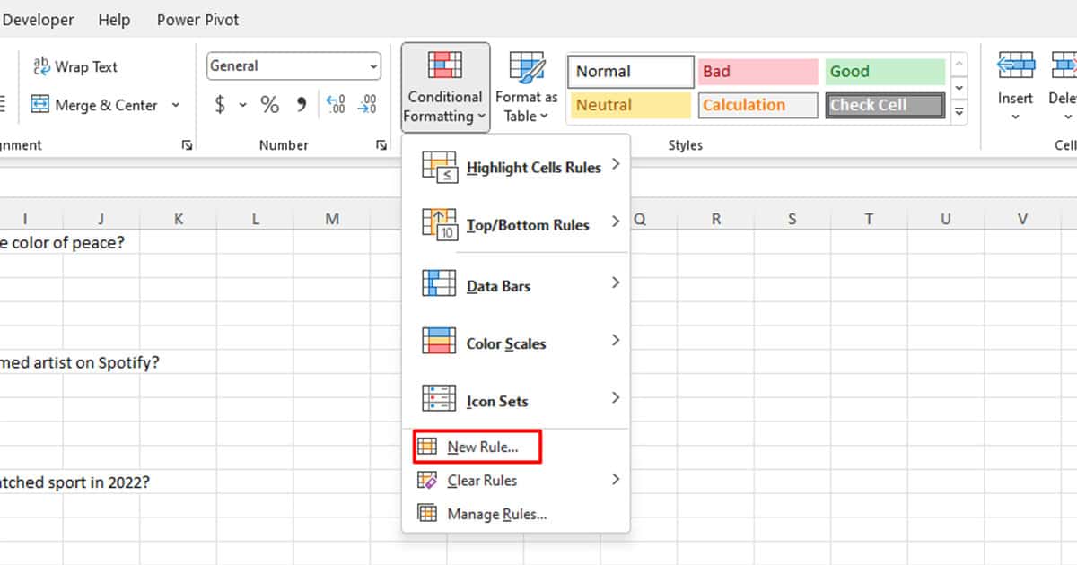
3. Choose Use a formula to determine which cells to format.
4. For incorrect answers, use this formula with the not equals to operator as a format to enter your condition:

=$C$13<>"Octagon"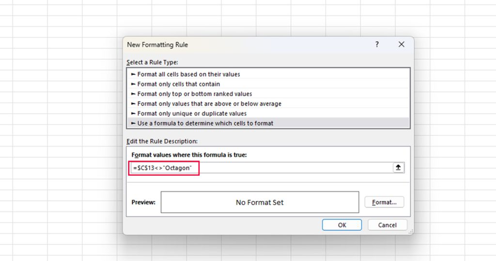

5. Click on the Format button.
6. Head to the Fill section and choose a fill color.
   
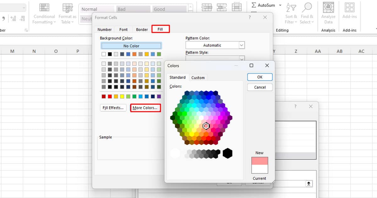
7. You can also choose to apply other formats from other tabs.
8. Click OK > OK.

Step 4: Change the Sheet’s Appearance

You can add icons and images onto your cells, or apply other formatting settings to make your sheet look more presentable. If you want to count the total number of correct answers, you can run the GET.CELL to count cells based on their color.

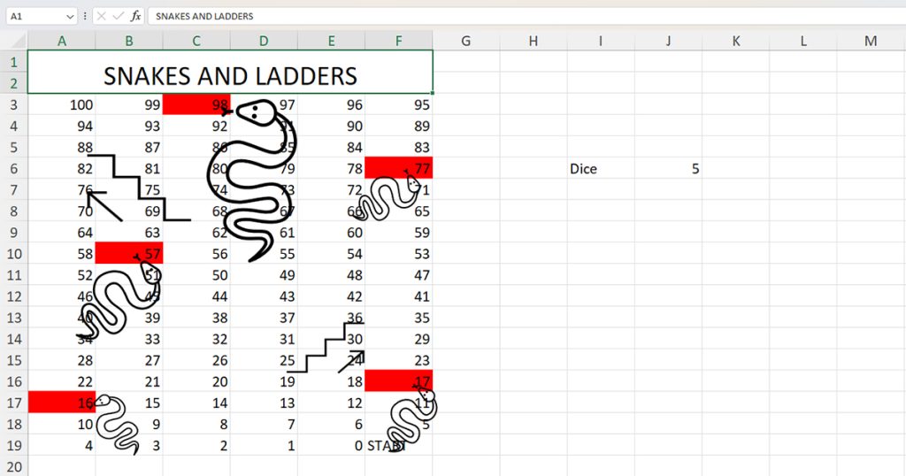
Snakes and Ladders

To create the Snakes and Ladders game, we will first create the game board and then use the RANDBETWEEN function for our dice.

Step 1: Enter Numbers

Enter 100 and 99 into the top two cells. Then. select these cells and drag the fill handle to 95.

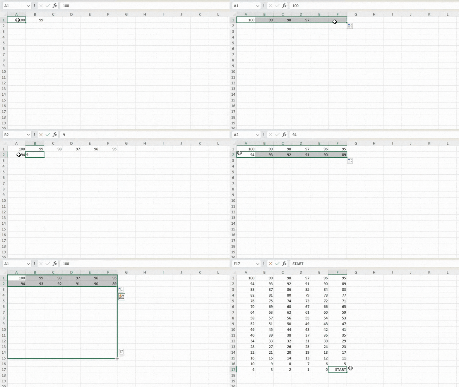
Repeat this at the bottom after entering 94 and 93. You can then select the two numbers from the range and drag the fill handle to fill in the rest of the numbers.

Step 2: Enter Snakes and Ladders

You can put icons for the snakes and ladders. Follow these steps to insert these icons in Excel:

1. Go to Insert.
2. In the Charts sections, select Illustrations > Icons.
   
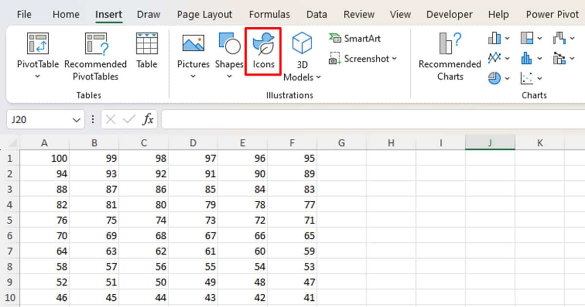
3. Search for Snake.
4. Select an icon and click Insert.
   
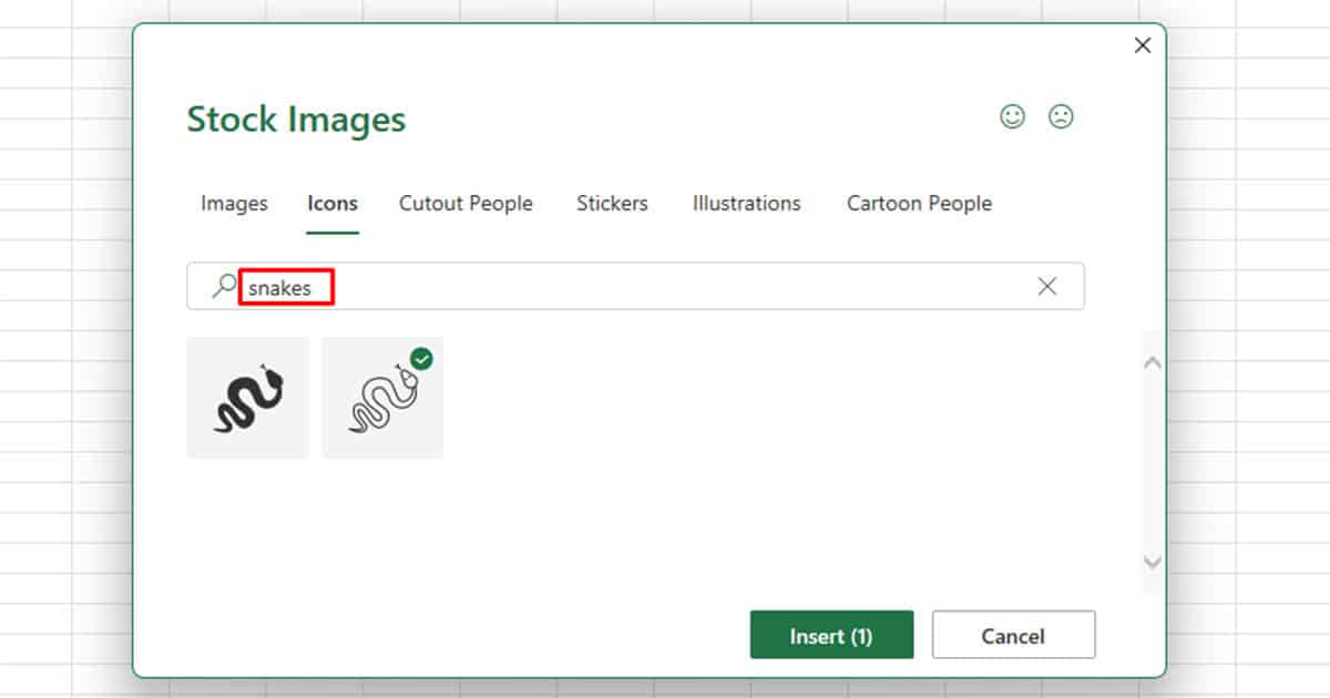
5. Resize the icon according to your convenience and place it on your board.
6. Use the copy-paste shortcut, (Ctrl + C/ Ctrl + V) to duplicate the icon.
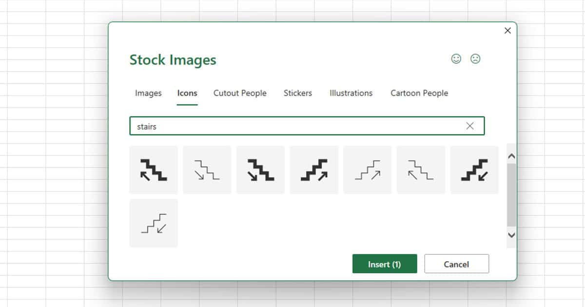
7. Repeat these steps to insert the stairs icon.
   

Step 4: Create a Dice

You can create the dice using the RANDBETWEEN function. As a dice contains numbers from 1-6, we will be setting our bottom value as 1 and top value as 6 in the RANDBETWEEN function.

=RANDBETWEEN(1,6)