In some of the advanced Excel formulas, you may have seen or used (–) double negative signs. It is widely popular in the SUMPRODUCT function.
What does double negative really do—and why are we using it? Does it make a difference in the formula?
Today, we will explore the rationale behind the Double Negative, also known as “Double Unary” in Excel Formulas.
What is Double Negative (- -) in Excel?
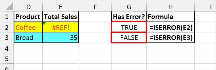
I believe you know that when using logical functions like ISNUMBER, ISERROR, etc, it results in a boolean value that is either TRUE or FALSE.
For example, if I use the =ISERROR(E2) formula, the formula returns TRUE because the cell contains a #REF error.
Similarly, when I enter, =ISERROR(E3)the outcome is FALSE.
Now, there can be instances when you would want these Boolean values to be numbers and perform calculations, be it to count cells on certain criteria, do conditional addition, or many more.
Well, that’s where the Double Negative (- -) comes in as a Knight in the Shining Armour for advanced formulas.
It basically coerces the TRUE value to 1 and FALSE to 0. So, instead of the boolean, your outcome would be either 1 or 0.
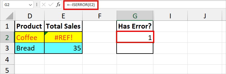
Again, let’s look into the same example as above but with the (- -) signs.
This time, if I enter =--ISERROR(E2), I’ll get 1.
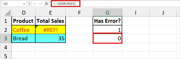
Likewise, for the FALSE condition, when I enter =--ISERROR(E3), I’ll receive a 0 value.
How to Use Double Negative in Excel—Examples
Above, I discussed a very basic usage of the Double Negative. Now, let’s go into more advanced examples.
Count Cells with Condition
SUMPRODUCT Function in Excel is simply used to multiply and add ranges.
But, if you put a Double Negative (- -) and tweak the formula a little, the formula becomes powerful and can sum cells based on criteria.
In short, you can count cell criteria like range (A2:A3 > B2:B3) with that formula.
So why not make the best use of this function using a double negative?
| Function | Syntax | Function Arguments |
| SUMPRODUCT | =SUMPRODUCT(array1, [array2], [array3],….) | array1: Range to return the product and add those results. [array2]: Extra ranges to multiply and add. |
Example:
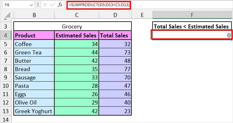
Here, in Column B, there are Product lists, Estimated sales numbers in Column C, and Total Sales values in Column D.
Let us count how many product quantities were sold for less than the estimated price (Total Sales < Estimated Sales).
To find out, this is the formula.
=SUMPRODUCT(--(D5:D13<C5:D13))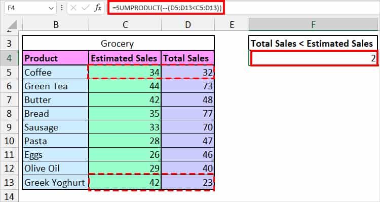
The formula returned 2. But, how did this actually happen? Let’s deep dive into it below. For that, I’ll be using the F9 key to debug the expression.
SUMPRODUCT(D5:D13<C5:D13): Suppose, you entered this formula without including the double negatives. It would obviously result in 0. Why?
This is because if you select the array D5:D13<C5:D13 and press F9, you’ll see that there are only TRUE and FALSE.
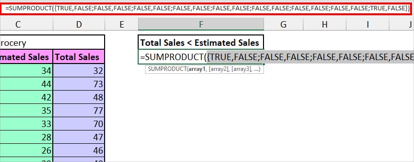
So, after using the (- -), all those Booleans will be 1 and 0 numerical values. When the SUMPRODUCT multiplies and adds, it returns the actual number as per the criteria which is 2 in our case.
Count Cells With Errors
Moving on, another application of the (- -) signs would be to count cells with errors. For that, I will nest SUMPRODUCT and ISERROR functions.
=SUMPRODUCT(--ISERROR(E2:E3))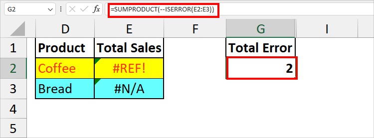
The formula counted and returned the total number of cells with errors which is 2.
Compare Columns and Count Matches
Suppose, you want to compare the values between two columns and count the cells that have the same value. Here, we will count the corresponding rows.
For that, I will again use the SUMPRODUCT function.
Example:
Let me compare the items in Column A and Column C. Here’s the formula I entered.
=SUMPRODUCT(--A2:A7 = C2:C7))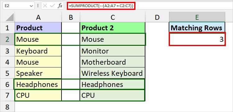
It returned 3 as an outcome.
Count Dates
Next, the SUMPRODUCT-Double Negative pair is also popular for counting dates in Excel.
But why opt for SUMPORDUCT instead of COUNTIF?
Well, there’s also a logic behind this. With the COUNTIF function, you would have to insert an extra helper column dedicated to weekdays.
On the other hand, you could dodge this step as the SUMPRODUCT function supports arrays.
As an example, I will count the number of dates based on the day of the week.
Suppose, I have lists of random dates in Column C. Similarly, I have Week Days name in Column E and day numbers in Column F.
To count, this is the formula I entered and copied it down
=SUMPRODUCT(--(WEEKDAY($C$2:$C$8,2)=F2))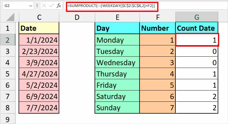
First, the WEEKDAY function counts the number of days and compares it with the number in F2. It results in a boolean array which is again converted by the double negative.
Finally, the SUMPRODUCT function adds the cells and returns the count for the Days.
Use SUMPRODUCT with Multiple Criteria
Until now, we just covered the examples for SUMPRODUCT and double negative with one criterion. But, the usage isn’t limited to it.
The best part is you can use it with the Multiple Criteria too.
Example:
Suppose, from the given dataset, I want to count the cells based on these two criteria.
- Total sales < estimated sales.
- Count only the cells with Coffee.
To do that, here’s the formula.
=SUMPRODUCT(--(D5:D13 < C5:C13), --(B5:B13 ="Coffee"))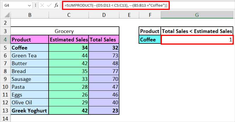
We got 1 as a result. Remember, – -(D5:D13 < C5:C13) is array1, – -(B5:B13 =”Coffee”) is array2 in the formula.