If you receive a #VALUE! Error, Excel is warning you that “The formula or cell references you’ve entered are wrong.” To be more straightforward, your formula contains an invalid data type.
Generally, your formula will result in a #VALUE! Error when there are,
- Unnecessary Spaces
- Formula Typos
- Hidden Characters
- Dates and Times in Text format
- Incorrect Array Dimensions
Since the error arises due to several factors, here, I have compiled the proven fixes to troubleshoot it.
Check and Change Formula
One of the main reasons you encounter the #VALUE! error could be because of the formula typo.
So, firstly, check the formula and make sure the syntax is correct. It should solve the error.
Here are a few things you could see.
- Ensure the function argument is separated by
,and not;. - See if you’re referencing the cell that contains the #VALUE! already. For instance, if there’s an error in the cell
C4, entering the=SUM(C2:C6)formula would result in the same #VALUE! Error. - Are there any text strings in the cell ranges? Since the functions discard Text for calculations, delete the words if you have any.
- Does your Formula support the specified arguments? For Instance, the IF function cannot take two “Test Criteria” at once. There’s an IFs function for it.
- In Lookup functions like VLOOKUP, XLOOKUP, and HLOOKUP, the column index must be 1. If there’s 0, change the argument.
- Opt for functions to perform calculations instead of arithmetic operators like
*, +, -,etc. Some functions are built-in in a way that automatically ignores the text values.
Match the Range in Formula
When you’re referencing the cell in array functions, the source and return range should be equal. If the two of them do not match, you will encounter the error.
So, look into your formula and ensure that the dimensions of ranges are neither greater nor less.
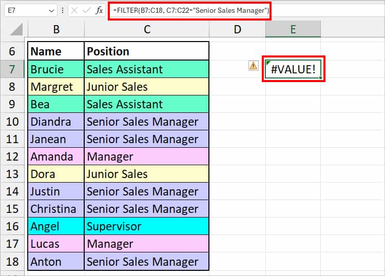
Let’s say I’m using the FILTER function to return all names for “Senior Sales Manager” from the lookup table.
When I entered =FILTER(B7:C18, C7:C22="Senior Sales Manager") formula, the outcome was #VALUE! Error. Why?
It’s because the C7:C22 range is greater than the B7:C18.
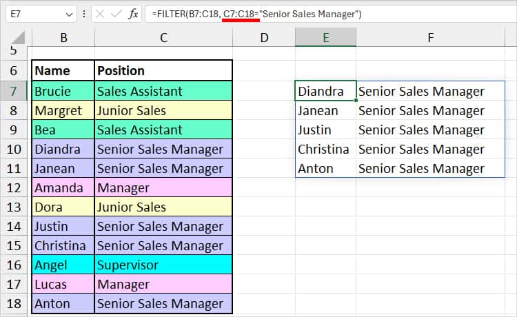
Here, the correct formula would be =FILTER(B7:C18, C7:C18="Senior Sales Manager"). Now, I have the results as expected.
Convert Date or Time Format
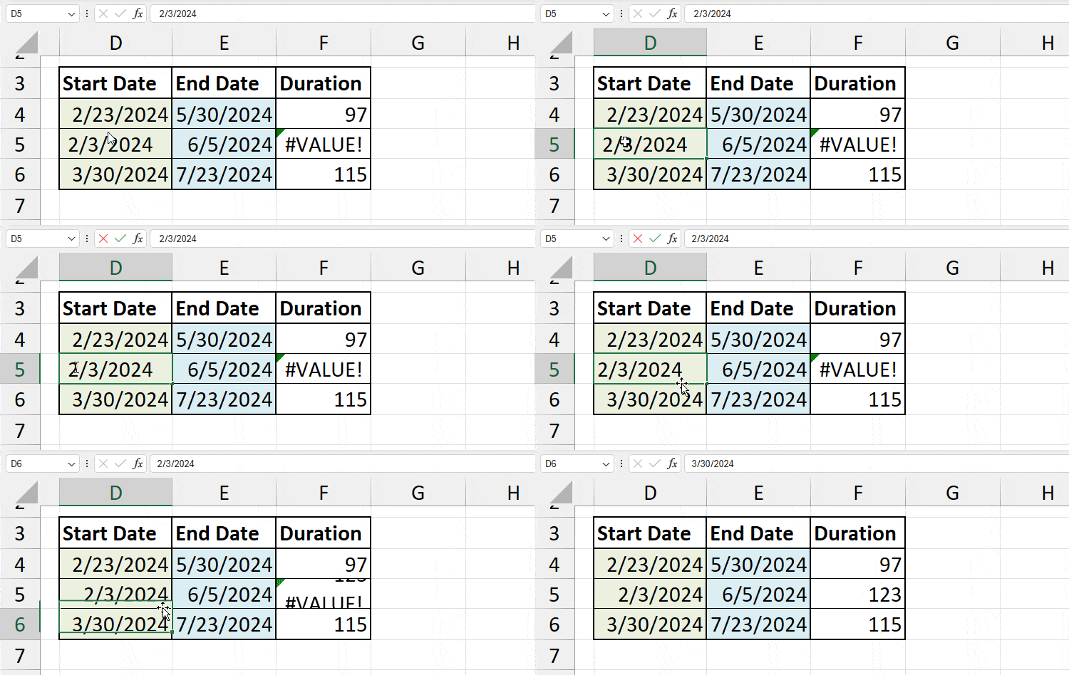
For dates and times, you will get #VALUE! Error when they are in the text format. In order to subtract or add dates/times, it must be in the Number format. So, verify how your data is stored and change it if required.
Leading Spaces or Apostrophes before the date and time make it a text. Remove those characters to change the formatting. The #VALUE! error should be gone.
Remove Spaces
Next, extra spaces also result in #VALUE! Error. Although it may not seem like a big deal, spaces convert your numbers to text format.
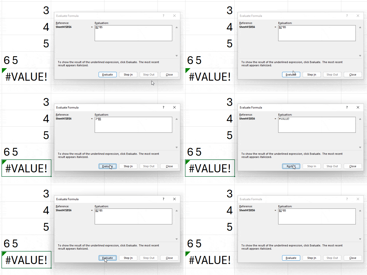
As you cannot detect spaces in a cell by yourself, you could use the Evaluate Formula to inspect.
Firstly, click the #VALUE! Error cell. Navigate to the Formulas tab and click Evaluate Formula.

On the dialogue box, hit the Evaluate button until you identify where it went wrong.
But, if you want to delete the unwanted spaces from your worksheet at once, you could opt for the Power Query tool.
- Select your data.
- Click Data Tab. Choose From Table/Range.

- In the pop-up, click Yes.

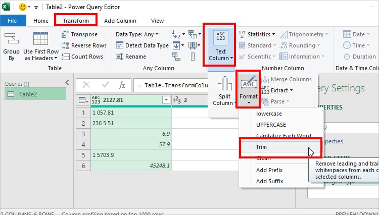
- In Power Query Editor window, head to Transform tab. Click on Text Column > Format > Trim.
- Go to Home Tab and select Close & Load.

Clear Hidden Characters
Do you have hidden characters in your cell? Sometimes, you may have null strings resulting from the formula that isn’t visible in the cell. Since such characters are invalid type, Excel sends you #VALUE! Error.
To remove them, select Empty cells and hit the Delete button.
Always make sure there’s a numerical value when you’re referring to a cell in the formula.
Use IFERROR Function
The IFERROR function doesn’t really solve the #VALUE! Error. However, you could use it to hide the error and replace it with any other text. It’s one of the best tricks to keep your spreadsheet free from errors and clean.
But again, I would recommend you use this only when you do not need to correct the error.
For Instance, let’s assume that I have dates in an incorrect format that’s resulting in the #VALUE! Error. Since I know the exact cause, I want the other users to take it as Invalid Dates.
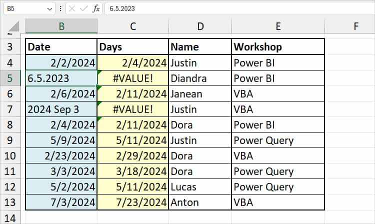
To substitute the error, here’s the formula I entered.
=IFERROR(DATEDIF(B4,C4,"d"), "Invalid Date")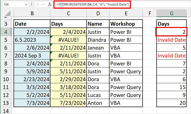
Here, the DATEDIF first returns the differences between the two dates. Then, if a cell has #VALUE!, the IFERROR results in the “Invalid Date.”