In Excel, Superscripts are commonly used during the data entry of scientific formulas, mathematical equations, Footnotes, Trademarks, Degree symbols, etc.
This font effect plays a huge role in the notation of values. For Instance, on number 12, if you change 2 as a superscript, it would be an exponential value of 1².
Unlike Microsoft Word or Google Docs, there’s no default Superscript button in the Font tab. Due to this, many of you might have been copying the superscript from an external source and pasting it onto the sheet.
But, in actual, Superscript is hidden in the Format Cells window. So, let’s learn how to superscript texts and numbers in this article.
Superscript for Texts
From Format Cells
Firstly, you can select the value and apply the Superscript effect from the Format Cells window.
Enter all the texts in the cell. Select the value you want to apply to the Superscript. Then, press Ctrl + 1 keyboard shortcut for the Format cells menu. Below, Effects checkmark for Superscript and hit OK.
Add Superscript to Excel Ribbon
The Format Cells menu is convenient only when you have smaller values. It can be monotonous when you need to keep opening the Format Cells window every time. So, let’s add the Superscript menu to the Excel ribbon.
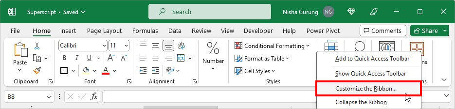
- Right-click on your Excel Ribbon and pick Customize the Ribbon.
- On Customize Ribbon, hover over the Home Tab and click on the New Group at the bottom.
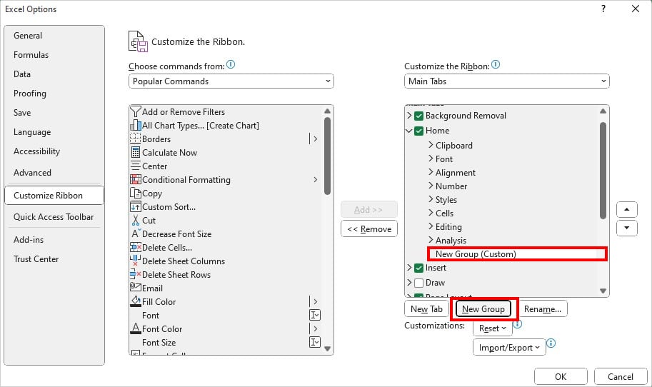
- From the Popular Commands lists in the left panel, select Superscript and click Add.
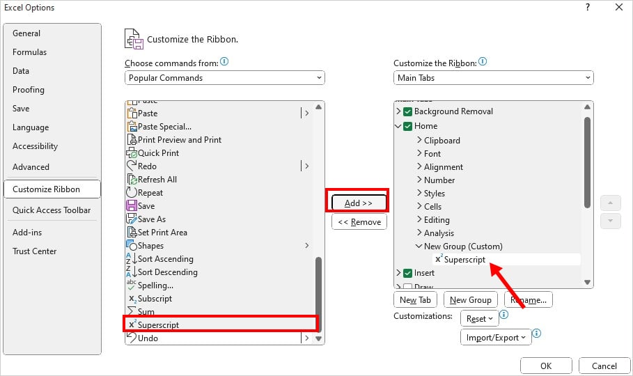
- Click OK.
- You’ll see the Superscript button in the New Group of Home Tab.
- To use it, select the values and click on the Superscript button. Or, you could also place the cursor, and hit the Superscript button. Then, start typing the values.
What I like most about this method is you can even use the Ribbon shortcuts to use the Superscript. Select the values and enter the given keys.
Shortcut: Alt, H, YFrom Quick Access Toolbar
Just like the Excel Ribbon, you can also add the Superscript command to the Quick Access Toolbar (QAT). If you prefer using commands from the QAT or wish to create your own custom shortcut to apply Superscript, go through these steps.
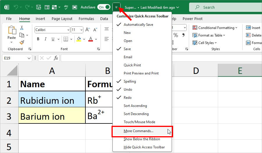
- Navigate to the Quick Access Toolbar.
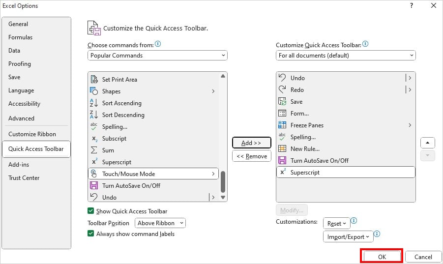
- Click on Customize Quick Access Toolbar > More Commands.
- On the lists of Popular Commands, choose Superscript and click Add button.
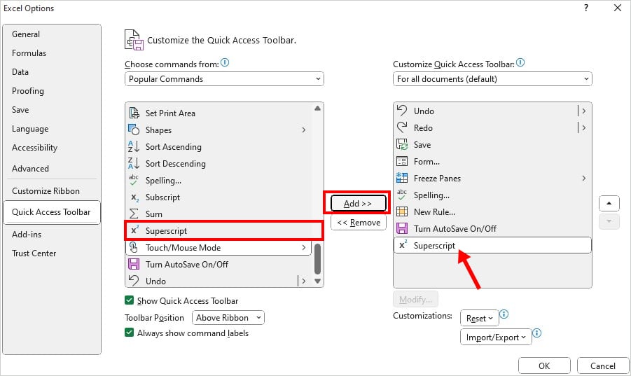
- Hit OK.
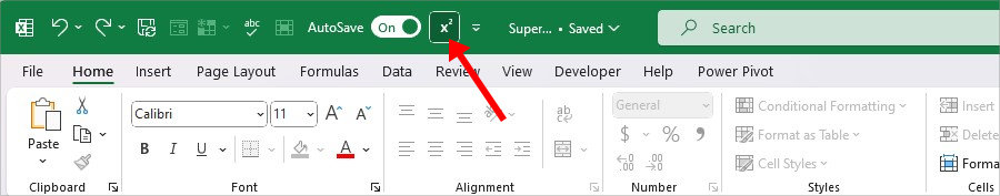
- Now, click on the Superscript command in QAT to use it.
Superscript for Numbers
While the Superscript buttons we’ve used above also work for the numbers, it will format the values as text strings. So, to calculate the numbers as an equation, we will use the Equation menu. However, if you want only the formatting, you could opt for the CHAR function, UNICHAR function, and Custom Number format instead.
From Equation
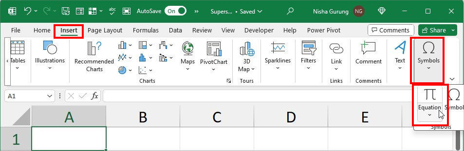
- Navigate to the Insert Tab.
- Click on Symbols > Equation.
- Now, on the Equation tab, click on Script. Then, choose any one Superscript format.
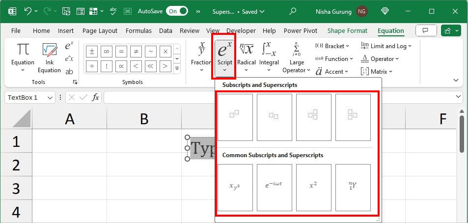
- Enter the Value.
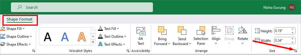
- Since the equation floats in the worksheet, go to the Shape Format Tab. On the Size group, click the Dialogue launcher.
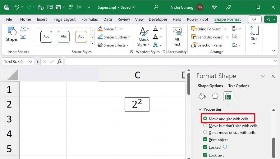
- Below Properties, choose Move and size with cells.
Using Ink Equation
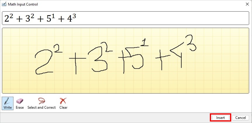
For longer equations, you can draw the formulas by yourself using the Ink Equation.
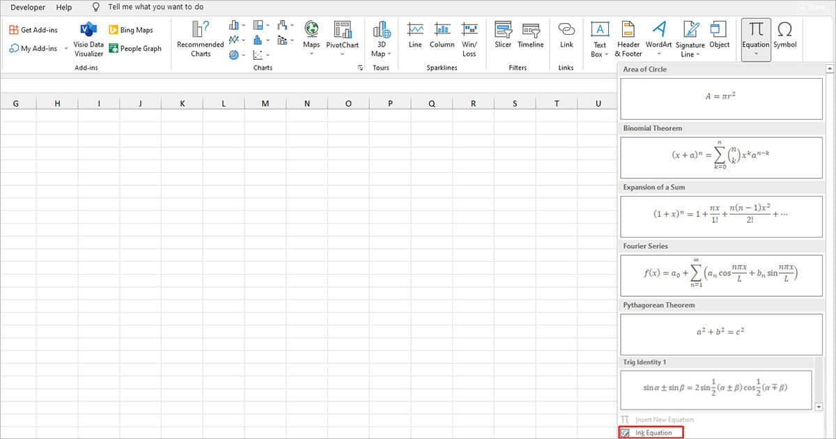
- Go to Insert Tab.
- From the Symbols group, select Equation > Ink Equation.
- Now, draw your equation with superscript. In case you made a mistake while drawing, use Erase, Select and Correct, Clear menu. Once you’re done, click Insert.
Using CHAR Function
Remember, the CHAR function returns the superscript in the text format.
| Number | CHAR code | Formula | Result |
| 1 | 185 | =A3&CHAR(185) | 1¹ |
| 2 | 178 | =A4&CHAR(178) | 1² |
| 3 | 179 | =A5&CHAR(179) | 1³ |
Use UNICHAR Function
CHAR function’s superscript code is limited to only 3 numbers. If you’d like to add more, you could opt for the UNICHAR function. With that said, this method is also used to change the number appearance only.
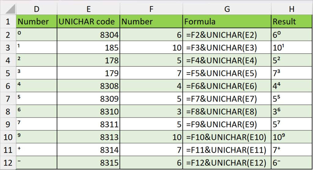
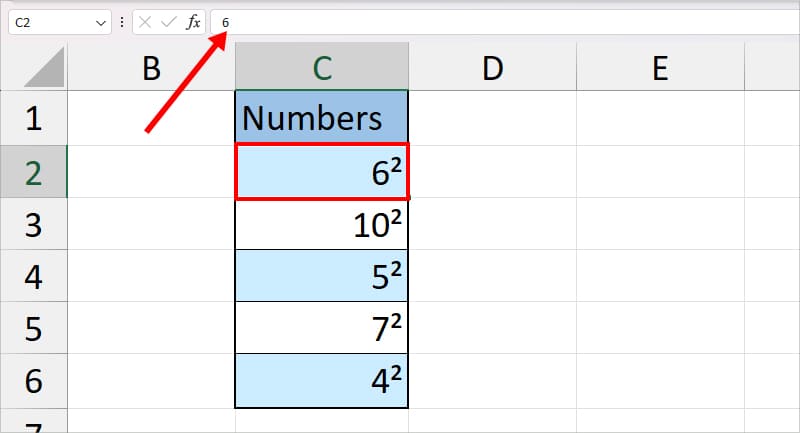
| Number | UNICHAR code | Number | Formula | Result |
| ⁰ | 8304 | 6 | =F2&UNICHAR(E2) | 6⁰ |
| ¹ | 185 | 10 | =F3&UNICHAR(E3) | 10¹ |
| ² | 178 | 5 | =F4&UNICHAR(E4) | 5² |
| ³ | 179 | 7 | =F5&UNICHAR(E5) | 7³ |
| ⁴ | 8308 | 4 | =F6&UNICHAR(E6) | 4⁴ |
| ⁵ | 8309 | 5 | =F7&UNICHAR(E7) | 5⁵ |
| ⁶ | 8310 | 3 | =F8&UNICHAR(E8) | 3⁶ |
| ⁷ | 8311 | 5 | =F9&UNICHAR(E9) | 5⁷ |
| ⁹ | 8313 | 10 | =F10&UNICHAR(E10) | 10⁹ |
| ⁺ | 8314 | 7 | =F11&UNICHAR(E11) | 7⁺ |
| ⁻ | 8315 | 6 | =F12&UNICHAR(E12) | 6⁻ |
From Custom Format
You can also create a custom format of superscript for your numbers. This method only changes the visual representation and not the actual value. Note that you need to use the Numpad of your keyboard to enter the Superscript code.
- Select the cell ranges and enter Ctrl + 1 for Format cells.
- Stay on the Number tab and go to the Custom category.
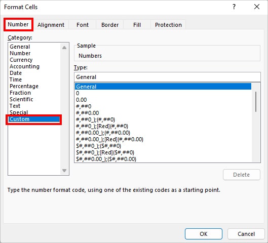
- On Type, enter 0. Then, while holding down the Alt key, enter a Superscript code. Here, I entered 1789 for ².
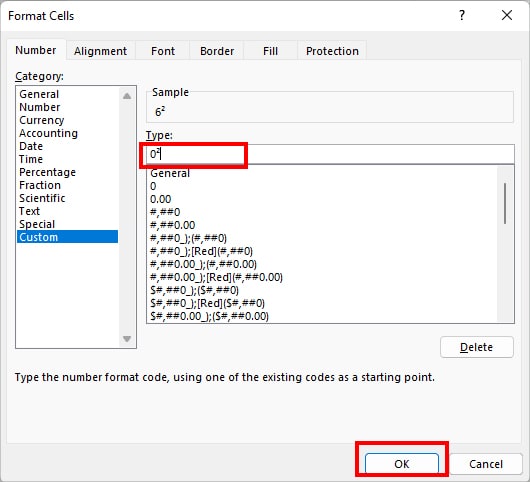
- Click OK. The numbers will have Superscript.