The LARGE function is one of Excel’s statistical functions. The name LARGE might trick many of you to think it’d return the largest number. But, there’s a MAX function built-in for this. So, the LARGE function actually returns the nth largest number from the cell ranges.
Using this function, you can exactly determine the 8th-highest number or 2nd-largest value from the dataset. It can be helpful if you need to identify the nth top scorers, nth longest time, sort numbers, and many more.
Arguments for LARGE Function in Excel
Excel’s LARGE function returns the kth maximum number from the data range.
Syntax: LARGE(array, k)These are the function arguments of a LARGE function.
- Array: Cell ranges to look for the largest value and return the kth position.
- k: Position number to return the largest number in. For eg: 2nd, 4th, etc.
Examples of Using LARGE Function in Excel
As an example, we have a list of numbers in Column B from cell B1:B8. Let’s find the 7th and 5th highest numbers using the LARGE function.
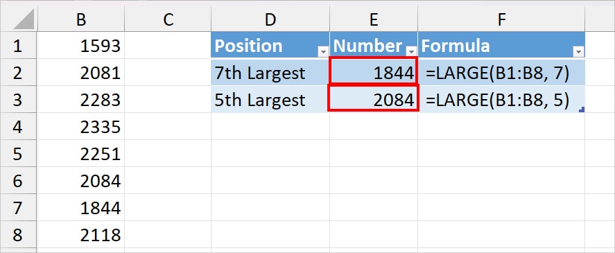
| Example | Formula | Result | Description |
| 7th Largest | =LARGE(B1:B8, 7) | 1844 | In the formula, we entered cells B1 through B8 as array and 7 as kth position. So, the formula returned the 7th highest number from the cell range. |
| 5th Largest | =LARGE(B1:B8, 5) | 2084 | This time, we just changed the value of k from 7 to 5 in the formula. So, it returned the 5th largest number. |
Applications of LARGE Function in Excel
Find Out Rank
Using Excel’s LARGE function is just the best way to calculate the nth ranks. For example, it could be the top 3 scores of a test, the top 5 salespersons with the highest sales, the top 2 employees with the highest salary, the top 4 winners in a race, and so on.
In the given example, we have the Students’ name and their Science test scores. Let’s say we want to find out the top 3 highest scorers. For each, we will enter a different kth value as in the table.
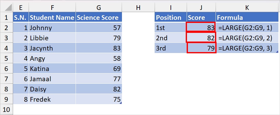
| Example | Formula | Output | Description |
| Highest Score | =LARGE(G2:G9, 1) | 83 | The formula returned the largest number from cells G2 through G9 as a result. This is because we entered the kth value as 1. |
| Second Highest score | =LARGE(G2:G9, 2) | 82 | Since we passed down 2 as k, the formula returned the second largest value which is 82. |
| Third Highest Score | =LARGE(G2:G9, 3) | 79 | In the formula, we specified 3 as the k argument. So, it returned the 3rd highest score from the G2:G9 score range. |
Calculate an Average of the Kth Largest Numbers
When you use the LARGE and AVERAGE functions nested together, you can calculate the average value of the kth largest numbers.
Example: We have lists of Teams and their Game scores in Column B and Column C respectively. Let’s find out the the Average between 2nd and 3rd largest scores. For this, the formula would be
=AVERAGE(LARGE(C2:C9, {2,3}))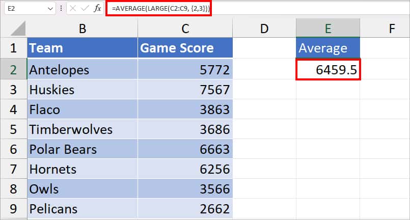
In the above formula, firstly, the LARGE function returns the 2nd and 3rd highest scores from the C2:C9 cell ranges which is (6663, 6256). Then, the AVERAGE function returns the average between these numbers which is 6459.5.
Sort Numbers in Descending Order
Another use of the LARGE function in Excel is to sort numbers in descending order. Now, you must think there’s a SORT function to do just that. But, as the SORT function is one of the new and dynamic array functions, LARGE functions can be useful on older Excel versions.
To do this, we will be nesting the ROW function inside the LARGE function.
Example: We have lists of numbers in Column B from cells B2:B8. To return them in the largest to smallest order, we used the following formula.
=LARGE($B$2:$B$9, ROWS($B$2:B2)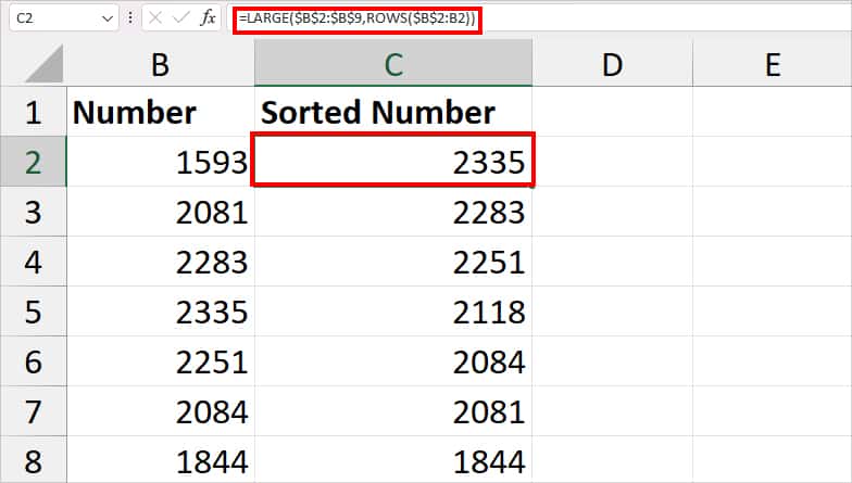
In the above formula, ROWS($B$2:B2) returns the total number of rows which is 1. Similarly, the LARGE function then takes ($B$2:$B$9) as array and 1 as k. Hence we got the largest number at first.
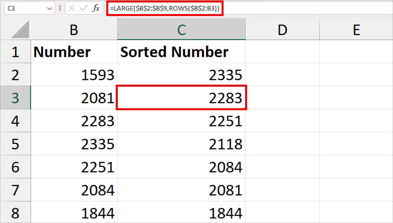
Now, when you copy down the formula, the value of k will be ROWS($B$2:B3). This is because we haven’t locked cell B2. So, it returns 2 rows. As a result, the LARGE function will return the second-largest number. This is how you get all of the numbers sorted in descending order.
Determine Longest Time
Just like how you can calculate the highest numbers from a range, it is also possible to find out the longest time from data. This is because Excel stores the time in decimal format.
Example: Here, we have a time duration for each participant in the Swimming competition. Let’s find out what is the 3 longest time duration to eliminate the participants in the next round. For this, again, we will use the ROW and LARGE functions together like above.
=LARGE($C$2:$C$8,ROWS($C$2:C2))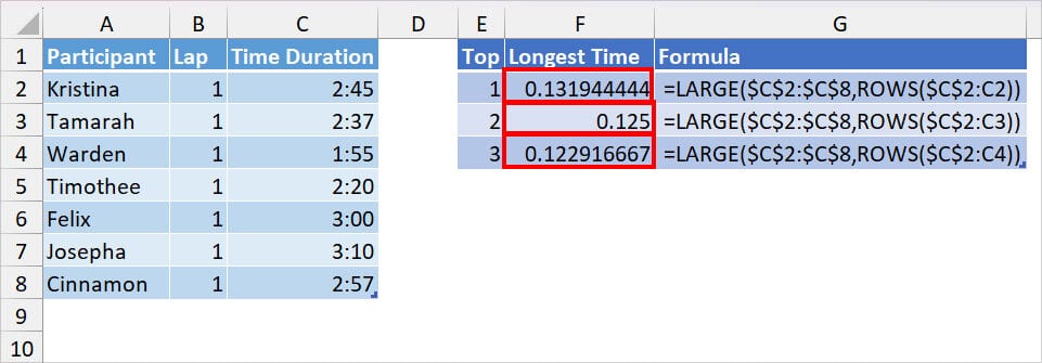
Once you get the result, use the Flash-fill handle to get the other two longest time. At first, the formula might return the output in decimal numbers.
During that case, you can change the number formatting to Time. For this, select the Numbers and go to the Home tab. From the Number group, pick Time from the drop-down list. So, the three longest time durations were 3:10, 3:00, and 2:57.
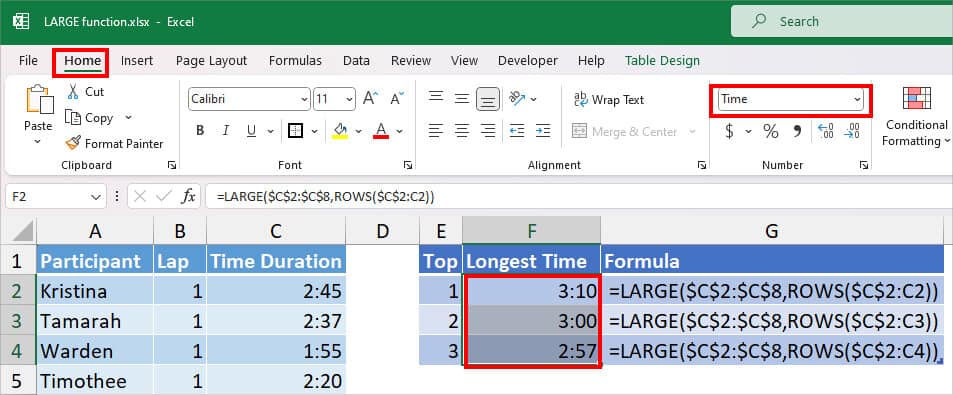
See how the formula works:
- ROWS($C$2:C2)): The formula first returns the number of rows between the $C$2:C2 cells which is 1.
- LARGE($C$2:$C$8, ROWS($C$2:C2)): The LARGE function then returns the 1st longest number from cell ranges $C$2:$C$8.
Avoid Errors When Using a LARGE Function in Excel
When using the LARGE function, these are the most common errors you may encounter. However, as long as you enter the correct argument in the formula, you can easily prevent these errors. See what each error implies in the LARGE function below.
- #NUM error: LARGE function will return the #NUM error if there’s no position to return to. Meaning, when the value of k > rank of numeric values or k ≤ 0 in a cell range. Likewise, another reason could be when the array you pass down in a formula is empty.
- #VALUE! Error: If you get #VALUE! Error in the LARGE function, it means that the array you enter in the formula contains non-numeric values.
Similar Functions Like LARGE Function
Excel has a MAX function which is similar to the LARGE Function. MAX function returns the largest number from a specified cell range without any position.
Syntax: MAX(number 1, [number2])Talking about the function arguments, you could enter multiple numbers (1, 3, 8, …..) as arguments or a cell range reference (C2:C8) to return the largest value from.