Need to sum data from multiple Excel sheets for that killer report but don’t know how? We’ve got your back. Whether it’s different months, dates, sales, currency, or anything else, we’ll show you how to add values in multiple sheets.
For starters, you could use the plus operator (+) to add the sheets like this (=Sheet1A1 + Sheet2A1 + Sheet3A1). But, as simple as it is for a smaller set of sheets, it could get exhausting for a large number of sheets.
So, we will be using Excel’s SUM, SUMIF, and nested functions to sum huge sheets in a more effortless way. These functions will create a dynamic reference of sheets such that the formula cell will auto-update whenever you change cell values.
Referencing Between Multiple Sheets
Before you start with the methods, it’s important you know how to reference the sheets first.
- Single Cell Reference: To reference a single cell of another sheet, enter the Sheet name like Sheet1!. Then, type in cell reference after the ! sign. For example,
Sheet1!A1, Sheet2!A3. - Range Reference: For range reference, you can use the (:) sign in the sheets too. Just like above, enter the cell range after the Sheet name. Examples:
- Cell Range:
Sheet5!A1:A10, Sheet10!A2:A5 - Name Range: For a named range, enter
Sheet1!NamedRange. Take, for instance, E16:E22 range is named “Total” and is your sum range for Sheet2. To reference it enter, Sheet2!Total. - Table Range: Remember, when you reference tables, it does not show the Sheet name in the formula. For table range, your cell referencing will be the table name and column header like this
Table1[Total]. But, if you’ve named a table, it’ll beCustomer_Table[Total]
- Cell Range:
- Relative Reference: Use Relative reference to change the cell location when copying down the formula. Sheet1!A1 or Sheet10!A2:A5 is a relative reference.
- Absolute Reference: Enter an absolute reference to lock the formula cell. It’ll help retain the original cell reference.
Sheet2!$N$2orSheet10!$A$2:$A$5is an absolute reference. - 3D Reference: When the sum range/cell is the same for all worksheets, it’ll create a 3-D reference. Example:
Sheet1:Sheet5!A1, Sheet1:Sheet5!A1:A3. - INDIRECT Function: Use an INDIRECT function to indirectly reference a cell/sheet in the formula. It’s especially helpful to reference the mass number of sheets. Suppose, in Sheet5, cell A2 contains sheet name “Sheet1,” B2 has Column “C”, and C2 has Row 5. If you enter,
=INDIRECT(“‘“&A2&”’” “‘!” &B2&C2), it’ll return the value of C5 from Sheet1. - External Reference: To reference sheets from another workbook, make sure the workbook is open first. Then, after you enter the formula, select the cell range of that sheet. Example:
[Book1]Sheet1!$E$2:$E$8
Using SUM Function
If you’ve used the SUM function to add random cells, you must’ve been already familiar with this function. Well, you could use the same SUM function to return the sum of multiple sheets.
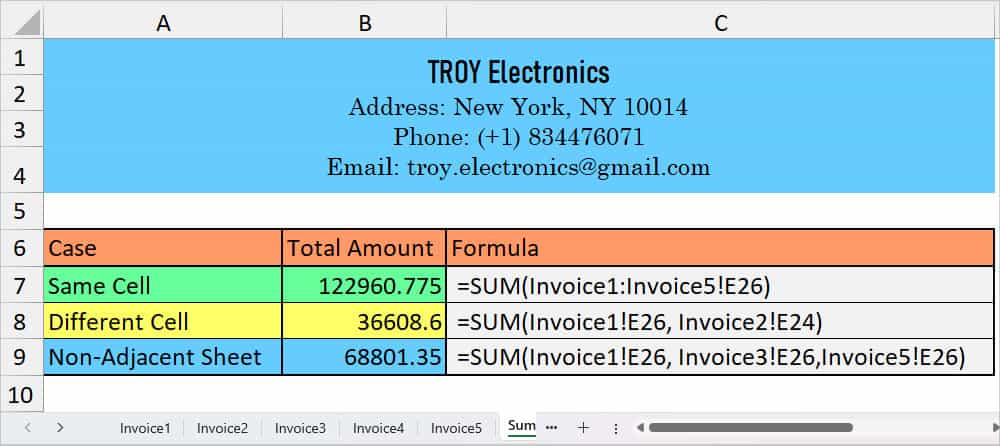
Example: Suppose we have 5 different sheets of invoices for TROY Electronics. We want to add the values of these sheets and return the result in the Summary Sheet. In the below table, we will be using the SUM function to add different Sheets in multiple cases.
| Case | Formula | Output | Description |
| Sum the Same Cells of Multiple Sheets | =SUM(Invoice1:Invoice5!E26) | 122960.775 | In the formula, we’ve passed down the argument to sum all E26 cells from Invoice 1 to Invoice 5. |
| Sum Different Cells of Multiple Sheets | =SUM(Invoice1!E26, Invoice2!E24) | 36608.6 | In this case, we’ve specified the argument to add cell E26 of Invoice 1 and cell E24 of Invoice 2. |
| Sum cells of Non-Adjacent Sheets | =SUM(Invoice1!E26, Invoice3!E26,Invoice5!E26) | 68801.35 | Here, we have entered the argument to add the same E26 cells. But, from Invoice 1, Invoice 3, and Invoice 5 which are non-adjacent sheets. |
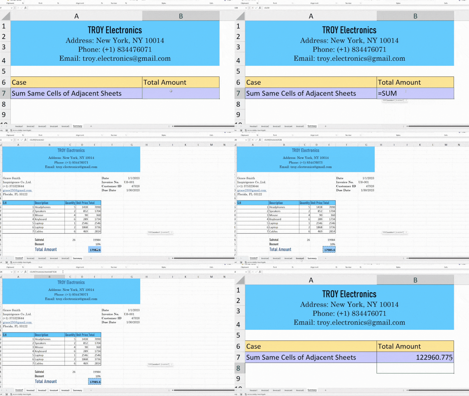
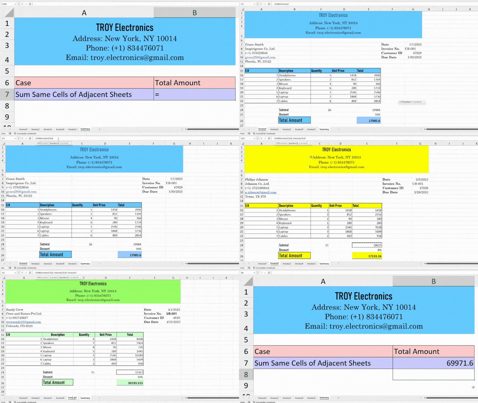
You could type all the above formulas manually or select the Sheets after entering =SUM(. I personally follow the latter method to avoid formulas typo. Here’re the tips you can follow.
- Firstly, enter =SUM(.
- Head to the First sheet and select a Cell. Then, do one of these.
- To select all adjacent cells, hold down the Shift button and click on the Last Sheet. When done, close the Bracket and press Enter.
- For non-adjacent sheets or different cells, enter a Comma after the First Sheet in the formula bar. Go to Another sheet and select a cell. After you select all sheets, close the Bracket and hit Enter.
- To select all adjacent cells, hold down the Shift button and click on the Last Sheet. When done, close the Bracket and press Enter.
Using SUMIF Function
If you need to sum ranges with criteria, there’s Excel’s SUMIF function to do just that. Unlike the SUM function, the SUMIF function does not support multiple sheets. So, here, we will add up each SUMIF function with the (+ operator).
However, I recommend you use this method only if you have limited sheets to add. From my experience, the formulas got extremely long in just 3 sheets.
Formula: =SUMIF(range, criteria, [sum_range]) + SUMIF(range, criteria, [sum_range]) + SUMIF (range, criteria, [sum_range]),......SUMIF Function arguments:
- Range: Cell range to apply the criteria to
- Criteria: Condition you want to set for the sum range
- Sum_range: Cell ranges you want to add
Example: I need to sum cell ranges from 3 sheets which are Invoice 1, Invoice 2, and Invoice 4 with different criteria for each. For this, I entered the formula as
=SUMIF(Invoice1!C16:C22, ">2", Invoice1!D16:D22) + SUMIF(Invoice2!C16:C22, ">1", Invoice2!D16:D22) + SUMIF(Invoice4!C16:C22, ">5", Invoice4!D16:D22)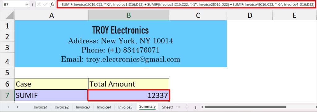
The formula returned 12337 as a result. Though the formula’s length looks scary, I assure you that we have only used the SUMIF formula to add three sheets with the plus operator.
P.S. We haven’t used the named range for cells in the formula to explain each argument as it could confuse the beginners. If you already have used SUMIF before, name the ranges to shorten the formula.
In the formula above, I used three criteria for each Sheet. Let’s check them out.
- SUMIF(Invoice1!C16:C22, “>2”, Invoice1!D16:D22): Firstly, for our Invoice 1 sheet, our criteria range is cells from C16:C22. As we’ve set the criteria “>2”, the formula will add all cell ranges of D16:D22 only if the value of C16:C22 is greater than 2.
- SUMIF(Invoice2!C16:C22, “>1”, Invoice2!D16:D22): For Invoice 2, the SUMIF function will only add D16:D22 sum range if the value of C16:C22 > 1.
- SUMIF(Invoice4!C16:C22, “>5”, Invoice4!D16:D22): In Invoice 4, the formula will add values from the D16:D22 range if the numbers of C16:C22 are greater than 5.
- In the end, the + operator adds up all returned values of these three sheets for the total sum.
Using SUMPRODUCT, SUMIF, and INDIRECT Function
While using only the SUMIF function is comparatively easier, it’s limited to adding only a few sheets. It would be a nightmare to select or manually type in the 10+ sheets in your SUMIF formula.
So, here, we will nest three different SUMPRODUCT, SUMIF, and INDIRECT functions to create an advanced formula. This is a little holistic approach for starters, yet a useful one for someone who has too many sheets to add.
Check out the syntax of each function in the table first.
| Function | Syntax | Description |
| SUMPRODUCT | =SUMPRODUCT(array1, [array2],…… | Adds the product of ranges or array. |
| SUMIF | =SUMIF(range, criteria, [sum_range]) | Adds cell ranges that meet the criteria |
| INDIRECT | =INDIRECT(ref_text, [a1]) | Returns the indirect reference of cell ranges that you specify by a text string |
Example: Let’s say we need to add the E16:E22 cell range from all 5 sheets with a certain condition. Our Sheets are named Invoice 1, Invoice 2, Invoice 3, Invoice4, and Invoice 5.
Before we begin, in the same formula sheet, I will first create a list of all Sheet Names in one column and Cell Ranges to add in another column. We’re doing this to make it easier to input the arguments of an indirect cell reference.
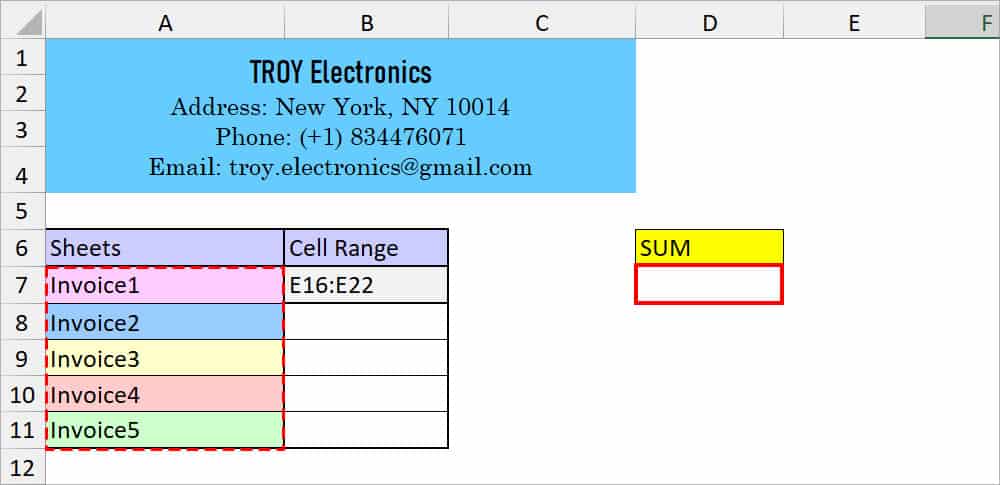
Now, in a new cell, I will use the given formula to return the sum.
=SUMPRODUCT(SUMIF(INDIRECT("'"&A7:A11&"'!"&B7), ">2"))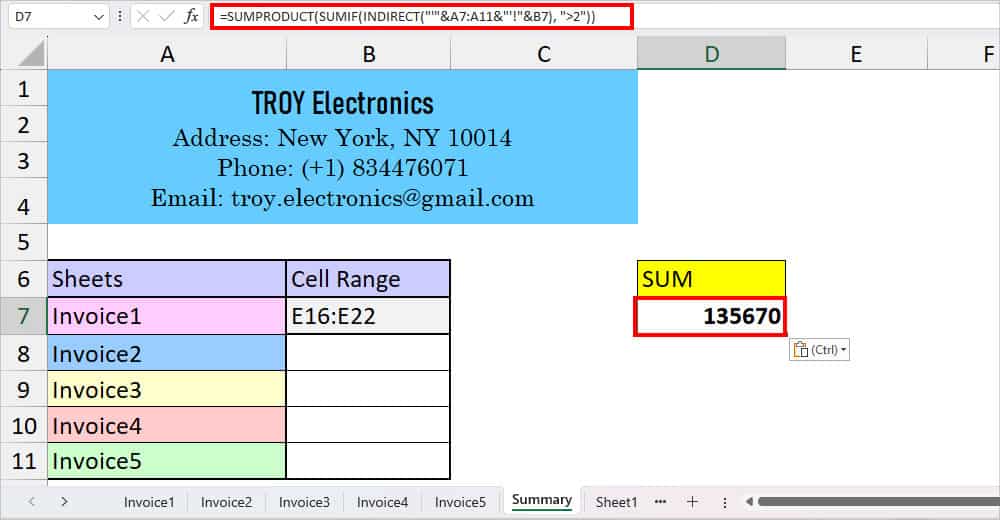
We got 135670 as a result. Now, let’s check each formula below.
- INDIRECT(“‘”&A7:A11&”‘!”&B7): This formula creates a 3-D range for cell E16 to E22 from Invoice1:Invoice5.
- SUMIF(INDIRECT(“‘”&A7:A11&”‘!”&B7), “>2”): The SUMIF function will return the sum range of E16:E22 of all 5 sheets whose criteria is “>2.” It returned the values of each sheet in rows.
- SUMPRODUCT(SUMIF(INDIRECT(“‘”&A7:A11&”‘!”&B7), “>2”)): Finally, the SUMPORDUCT function adds the returned array of a sum. Thus, we will have a total value in cell D7.