How to Separate Names in Excel

While working in Excel, you might come across a list of names that need to be split into multiple columns like First Name, Middle Name, and Last Name. Manually separating each of them is inconvenient and can take up too much time, especially if the list is too long. Imagine having to separate a list of thousand names!

Fortunately, there are efficient ways to ease the process. However, all the names you want to convert should preferably follow a similar pattern, like all the names separated with a comma or space for a better result.

Using the Text-to-Columns Feature

Text to Columns is a powerful Excel feature that can separate all your full names into separate columns. It doesn’t involve using any complex formulas and even provides a preview of the output.

The way it works is by using the delimiter, that exists on the data. In our case, anything that separates the names can be used as a delimiter.

For instance, if the name is “Jack John Reacher”, the delimiter is the space character. But, if the name is “Jack+John+Reacher”, the delimiter is the plus symbol.

Also, there can be multiple delimiters in a name. For instance, in the name “Jack, John Reacher”, there are two delimiters; Comma and Space.

To use the feature,

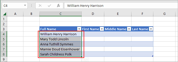
Select the cell (s) containing the names you want to separate.
Go to the Data tab.
Then, click Text to Columns under the Data Tools section.
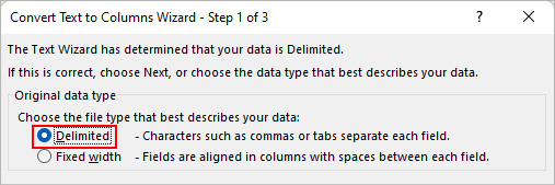
On the next window prompt, choose Delimited and click Next.
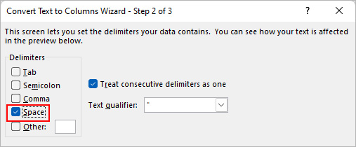
Under the Delimiters section, choose the appropriate delimiter according to the following cases.
- Single Delimiter: Choose one of the provided options (Tab, Semicolon, Comma, Space). If your name is separated by a character other than the available options, you can choose Other and input it there.
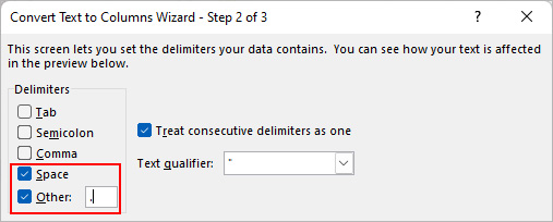
- Multiple Delimiter: If you have multiple delimiters, enable multiple options. For instance, if your text is “Jack Jr. Reacher”, choose the Space option and enter the full stop character. next to others.
Enable the Treat consecutive delimiters as one checkbox.
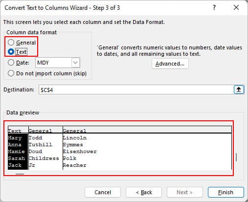
Since we are looking to separate a name, choose Text or General in the next window. Also, take a look at the final output preview and check if it’s what you want.
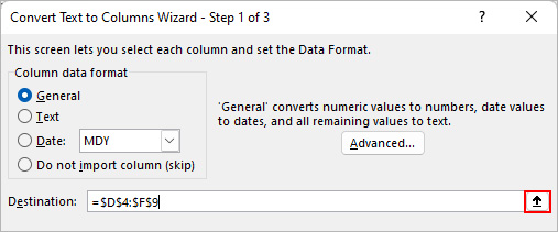
Click the Up arrow icon at the end of the Destination textbox.
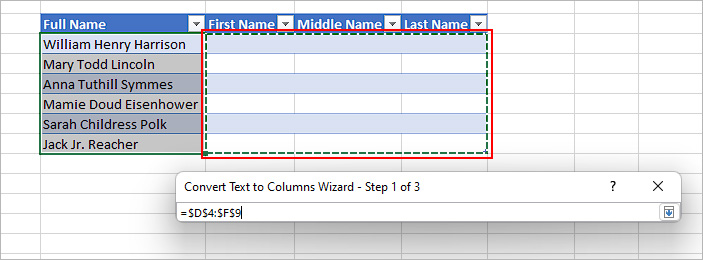
Select the cells where you want the final separated names output.
Click Finish.

Using the Autofill Feature

If the names and output columns are already in the table format, you can easily separate them using the Autofill feature. Even if they aren’t, you can easily turn them into a table. Then, you can use the autofill feature to separate the names.

Highlight the names column along with columns where you want to display the separated text.
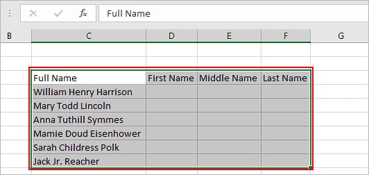
Then, press Ctrl + T to convert them into a table.
Now, manually enter your first name under the appropriate column. Here, it’s below the First Name column.
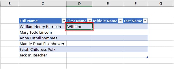
Then, press Enter to go to the next row and immediately type the first name for the next first name. Press Enter once you see the autofill suggesting the respective first name results in other rows.
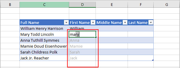
Similarly, repeat steps 3 and 4 to fill in the other names. (Middle name and Last name).

Note: If you missed the autocomplete, press Ctrl + S to save and try again.

Using Power Query

Power Query is quite similar to the Text to Columns feature. It also uses delimiter (s) to separate text into columns. However, after it splits the text, the output is provided in the table format, which makes it even easier to sort the names alphabetically or according to color.

Select the cell (s) which contain the names data.
Go to the Data tab.
Select From Table/Range inside the Get& Transform Data section.
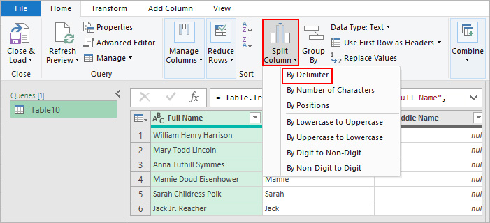
Select Split Column and choose the By delimiter option under the Home tab.
Then, on the Split Column by Delimiter prompt, choose the correct delimiter according to the names data. If the preferred delimiter isn’t available in the options, choose Custom and enter the delimiter in the empty text box below.
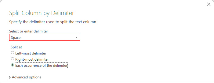
Under the Split at section, choose Each occurrence of the delimiter.
Expand the Advanced options.
By default, the output will be split into columns. But if you want the output in row format, select Rows. Also, choose the number of columns you want the full names to split. For instance, if the full name contains three names, choose 3.
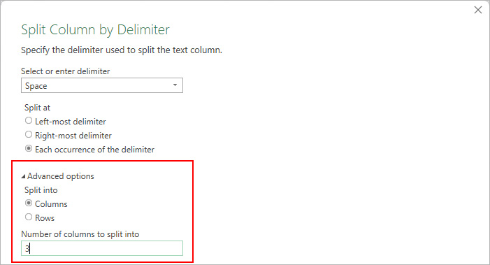
Click OK.
Check the preview and click Close & Load in the top left corner.
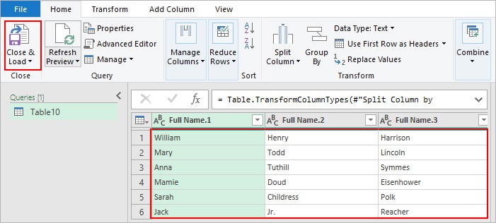
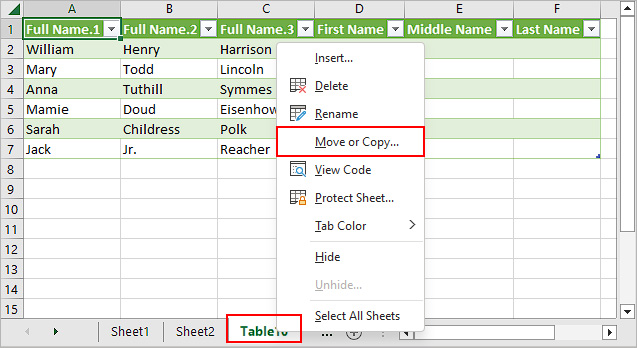
By default, Excel places the output in the new worksheet. But, you can copy or move it to any other sheet. Just right-click on the sheet with the output, and select Move or Copy. Then, choose the sheet you want the output.

Using the Textsplit Function

If you are using Excel with Microsoft Office 365 or online, you have a separate function called “TEXTSPLIT”. It’s much like the combination of the text-to-columns feature and the Excel formula.

Syntax:

=TEXTSPLIT(text, column_delimiter, [row_delimiter],[ignore_empty], [match_model], [pad_with])

Since we are trying to separate only the names, the most essential arguments are as follows.

text: text you want to separate
column_delimiter: list of delimiters that repeat on your texts

Convert the data and the output columns into a table so that you can easily sort the data later. You can do that by selecting them and choosing one of the formats under Format As table.
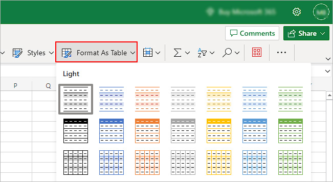
Select one of the cells in a column where you want to extract the first names. Then, type the following
=TEXTSPLIT(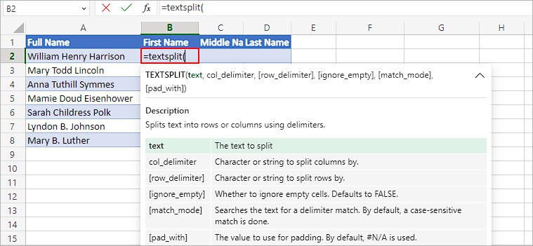

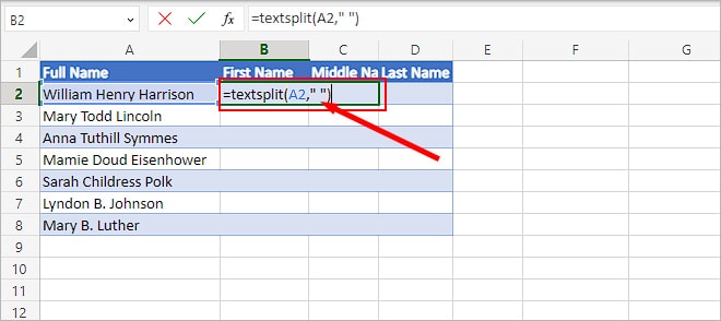
Now, select one of the cells which contains the full name, preferably the first cell in the names list.
Then, enter the delimiter inside the double quotes and close the bracket.
If you have multiple delimiters, enter them inside the double quotes and separate them with a comma. Then, enclose them inside a curly bracket. For instance, =TEXTSPLIT(A8,{" ","."})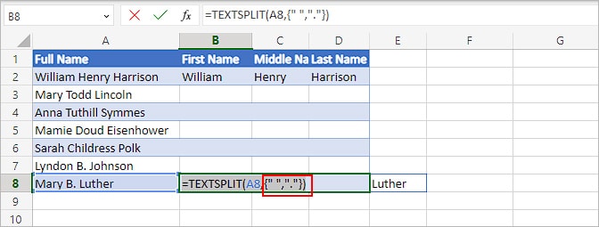
Add a parenthesis to close the formula and press Enter.
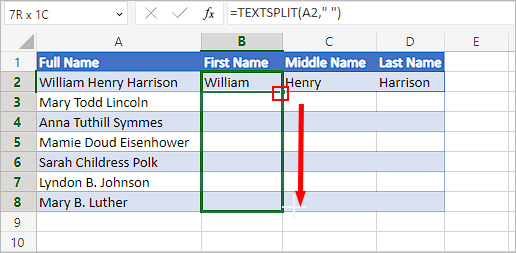
Once you have the first output, select one of its cells and drag down the corner handle across the rows containing the remaining names. Other columns will also be filled automatically given that you have converted the names data into a table.

How to Separate Names that Don’t Contain a Delimiter?

All the above methods rely on the occurrence of at least one delimiter such as space, comma, or something similar. But what if your “names” data doesn’t contain such delimiters?

For instance, one such name might be of the format; JackSmith.

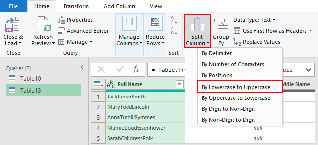
To separate such names, you can use Power Query. Unlike the previously used Delimiter option, we use the LowerCase to Uppercase option here. This is because the last letter of the first name ends in lowercase (JackSmith) and the last name starts with an uppercase character (JackSmith).

Select the column with full names.
Under the Data tab, click From Table.
Once your data loads into power query, select Split Column > By Lowercase to Uppercase.
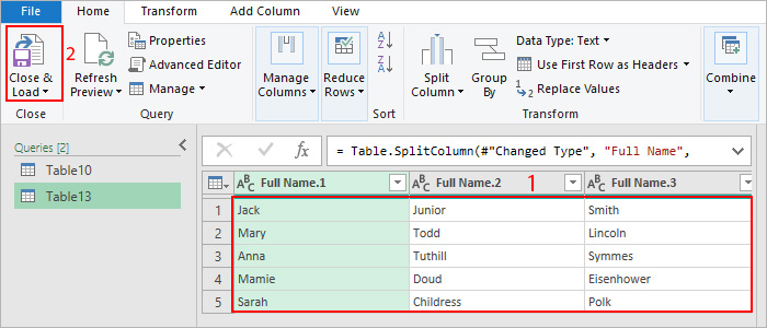
While on the same Power Query window, check if you have the desired result. Then, click Close & Load.

Using an Excel Formula

The above methods are quite simple and more effective than an Excel formula to split texts. Nonetheless, if you are familiar with using Excel formulas, you can use them to separate several texts that have very unique formats.

Before moving on, it’s helpful to know that an Excel formula always evaluates the innermost function first and then starts spreading onto the outer functions.

Step 1: Extract the First Name

=LEFT(A2, SEARCH(" ", A2,1) -1)

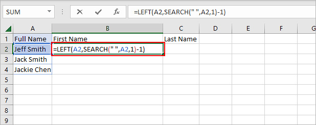
Here, we are extracting the leftmost part (Jeff), which is the first name in our case. Now, the formula SEARCH(“ “, A2, 1) searches for a blank space from the first position of the text in the A2 cell. Then, the search function returns the total number of letters in the text excluding the space character.

Now, we get =LEFT(A2,7). This formula extracts the first seven letters of the text, which is William from the selected cell A2.

Step 2: Extract the Last Name

=RIGHT(A2, LEN(A2)-SEARCH(" ", A2,1))

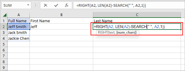
Here, we are extracting the last name using the RIGHT function. The formula LEN(A2) simply gives the length of the text in the A2 cell and returns 16 as output. And, the SEARCH(“ “, A2, 1) searches for a blank character starting from the first letter of the A2 cell and returns 8 as output.

Now, the formula is =RIGHT(A2, 16-8), which is equivalent to =RIGHT(A2,8). And, the =RIGHT(A2,8) returns the eight rightmost characters, which evaluates to Harrison.

Step 3: Use the Autofill Feature

Drag down the corner handles for the output of the first name and last name to fill the necessary rows.