Does not equal sign (<>) is one of the comparison operators that result in logical value like a TRUE or FALSE when comparing the two items. Basically, if one value does not equal another, you’ll get TRUE. Likewise, if the value matches, it’ll return FALSE.
Although the <> might not be the most used comparison operator, it has a wide range of applications in Excel. You can use it solely to determine the not equal to value with True or False. Or, use this operator with other Excel functions like COUNTIF, IF, SUMIF, etc to set criteria for the logical test.
Things to Note When Using Does Not Equal Sign <> in Excel
- You must enter at least two values to use the <> operator.
- The <> operator is case-sensitive. For instance, if you enter “Excel”, it’ll return TRUE if the value in the cell contains “excel” which is in lowercase.
- When you pass down an item in the formula, you must double-quote the value. If you don’t, you’ll get the #NAME? Error.
Examples of Using Not Equal Signs in Excel
You can use the not equal operator <> with cell references, values, booleans, etc. Let’s check out all of them with the basic examples in the given table.
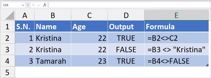
| S.N | Example | Formula | Result | Description |
| 1 | Cell reference | =B2<>C2 | TRUE | In this example, we are using the <> operator to check if the value of cell B2 is not equal to C2. Since the values do not match, it returned TRUE. |
| 2 | Value | =B3 <> “Kristina” | FALSE | In the formula, we entered the value “Kristina” to see if the item in cell B3 does not match it. Since the value was equal, it returned FALSE. |
| 3 | Boolean | =B4<>FALSE | TRUE | Checks if the value of B4 does not equal to FALSE. Returns TRUE if there is a different item. Similarly, returns FALSE, if the cell B4 contains FALSE. For booleans like TRUE or FALSE, you do not have to enclose them inside the double quotation mark. |
Using Does Not Equal Signs With Excel Formula
<> with IF Function
When solely using the <> operator, you’ll either get TRUE or FALSE. But, if you use the IF function with <>, you can specify the logical value to return a different result. For Instance, return Yes or No instead of TRUE or FALSE.
Example: Here, we have several name list and their ages in Columns A and B. Suppose, the Age Criteria is 22. Using the IF and <> operators, let’s find out if the participants are eligible or not. For this, we entered the formula as
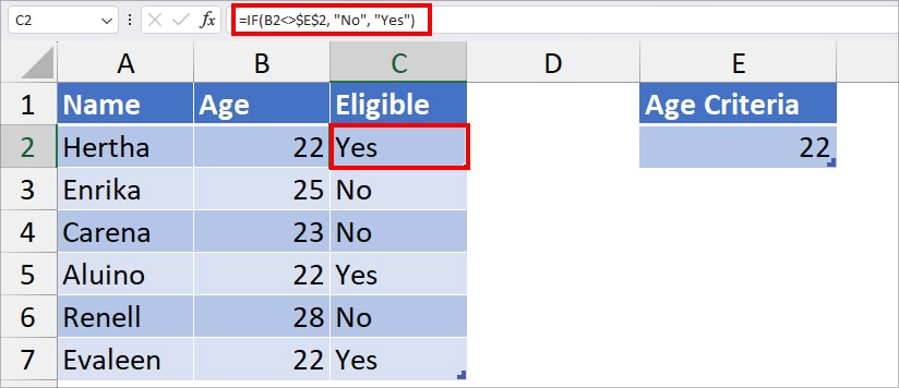
=IF(B2<>$E$2, "No", "Yes")In the above formula, we have passed down the criteria as B2<>$E$2. We locked the cell E2 making it an absolute reference to copy the formula to other cells.
If the value of B2 is not equal to the value of E2, it’ll return No. However, if the value of B2 and E2 match, the formula will return Yes. In our case, it returned Yes. We then used the flash fill to fill data in other cells.
<> with COUNTIF Function
Does not equal to operator <> can be best used with Excel’s COUNTIF function. The COUNTIF function counts and returns the total number of cells within the specified range in a given criteria. You could use the <> operator to specify the not equal to this or that condition while counting cells. For Instance, count cells not equal to blank cells, cells not equal to pending, etc.
Example 1: Count Non-Blank Cells
If you have empty cells in your data but wish to count only the non-blank cells, here’s the formula you can use
=COUNTIF(B3:H14,"<>"&"")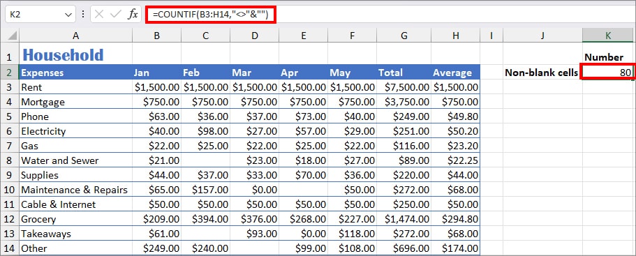
In the above formula, we have passed down “<>”&”” criteria which means not equal to blank cells “”. So, the formula will count all the non-blank cells from cell range B3 through H14. Then, returned 80 as an output.
Example 2: Count Completed Cells
We have a list of Completed and Pending statuses in Column E. Suppose we want to count only the cells with completed. For this, we entered the formula as
=COUNTIF(E2:E13, "<>Pending")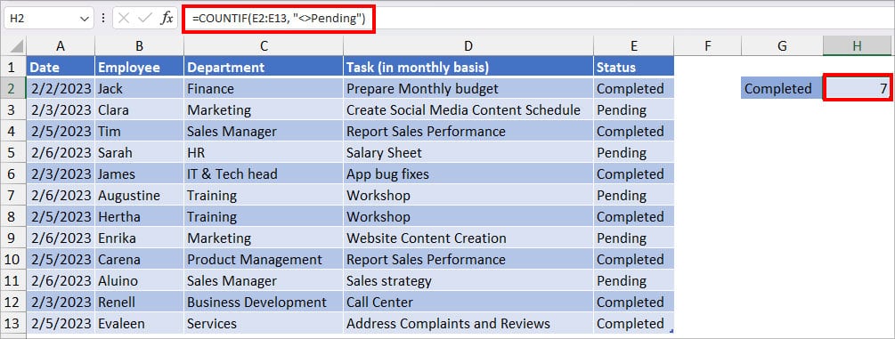
In this formula, we have specified the “<>Pending” (does not equal to Pending) criteria. So, the COUNTIF function returns the total number of Completed cells from E2 through E13 cell range. As a result, we got 7.
<> with Conditional Formatting
You can use the <> operator in the Conditional Formatting formula to highlight the cells not equal to a specific item.
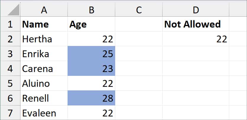
Example: Suppose, you want to highlight the cells of Column B whose value does not match with cell D2.
- Firstly, select the cells to highlight data.
- From the Home tab, click on Conditional Formatting and pick New Rule.
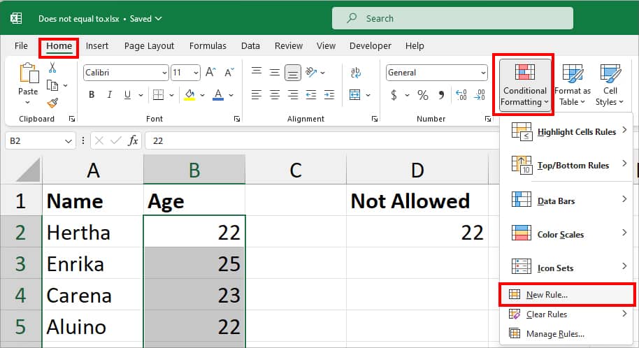
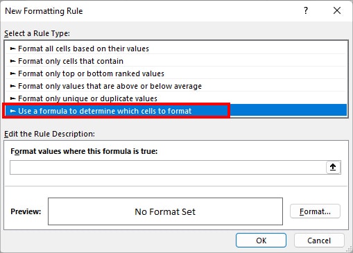
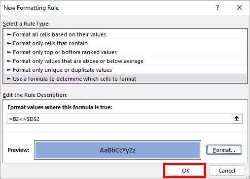
- On the New Formatting Rule window, click Use a formula to determine which cells to format.
- Enter
=B2<>$D$2formula in the box. Then, click on Format.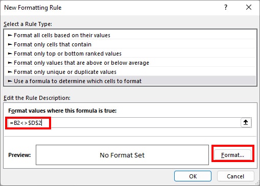
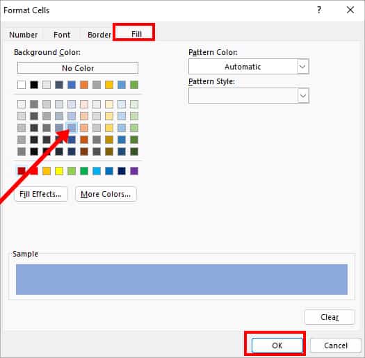
- On Format cells, head to Fill tab and select a colour to highlight the cell with. Hit OK.
- Click OK.
- =B2<>$D$2 formula will highlight all cell that does not match with the value in $D$2.
<> with SUMIF Function
If you want to exclude certain items to calculate when using the SUMIF function, you could create criteria using the <> operator.
Example: Let’s find out the SUMIF value of January Month without the value of 200. To do so, we entered the formula as
=SUMIF(B2:B6, "<> 200")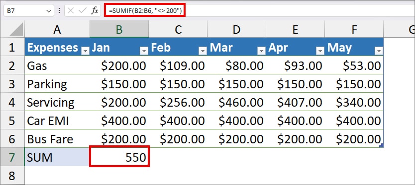
In the above formula, we set the criteria to sum the cell ranges B2:B6 that does not equal 200(“<>200”). So, after excluding the value of 200 from the data, it returned 550 as an output.
Alternative to Does Not Equal to <> Operator
Excel has a NOT function which is just the formula version for the <> operator. The NOT function returns TRUE if two values are not equal and FALSE when the two values match. While the <> operator is simple to use, the NOT function can be a better alternative when it comes to nesting the logical functions together. NOT function only has logic as an argument.
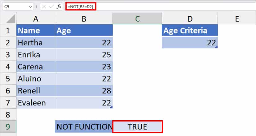
Syntax: NOT(logical)For example, if I enter the =NOT(B3=D2) formula, it’ll return either TRUE or FALSE. As the value of B3 is NOT equal to D2, the formula returned TRUE.
