In Real Life, Scientific Notations are used to express big numbers in a more compact form for calculations.
For example, in the Physics problems, it is easy to express that the length of a lake is 1.78 * 10 ^ (11) m rather than 178000000000.00 m.
In addition to solving such Physics, Mathematical, or Engineering problems in Excel, formatting numbers in the Scientific Notation is also one of the best ways to avoid the #### error. In this format, you can shorten and fit all values in a cell without expanding the Column Size.
Personally, whenever I need to use the Scientific Notation, I quickly select the number and press Ctrl + Shift + ^ keyboard shortcut. However, we also have other ways to change the formatting in different instances.
Besides, if needed, you can always avoid Excel from automatically converting values into Scientific notation.
Format Numbers as Scientific Notation
From Home Tab
For users who aren’t much used to the keyboard shortcuts, you can change the number formatting to Scientific Notation from the Home Tab.
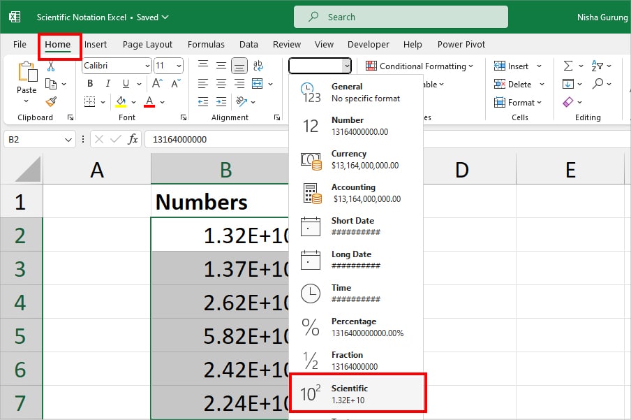
To do that, select the Cell Ranges with Numbers. Expand the drop-down menu in the Number Section and choose Scientific.
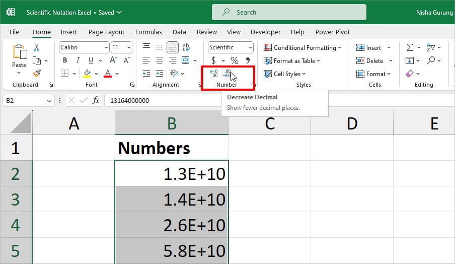
After that, use the Increase Decimal and Decrease Decimal buttons to change the Decimal Places.
From Format Cells
While it’s quicker to apply Scientific format from the Home Tab, you’ll only have a default format with 2 decimal places.
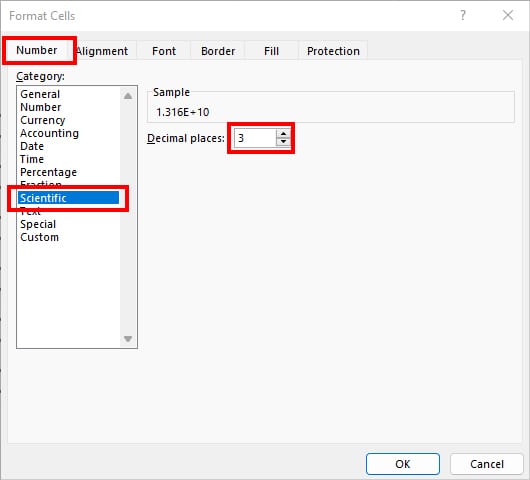
So, if you want to specify the decimal digit or create your own custom Scientific format, you can do it from the Format Cells window.
- Select Cell ranges and press Ctrl + 1 for the Format Cells window.
- Stay on the Number Tab. Then, perform any one of these steps.
- Click on Scientific Category. On the Decimal Places, enter Number.
- Go to Custom Category. On the Type field enter
“0.0E+00”or“0.00E+00.”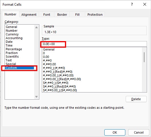
- Click on Scientific Category. On the Decimal Places, enter Number.
- See the sample of Scientific Number Format. Once you’re done, hit OK.
Using TEXT Function
Next, you can also use the TEXT function to format numbers as Scientific. This method is helpful when you want to keep the original data as well as have Scientific notation in a new cell.
But, keep in mind, as this function returns results in text format, the numbers will no longer be useful for calculations. It is mostly used to convert the number to text.
Syntax: TEXT(value you want to format, “Format to apply)Example:
Suppose I have lists of numbers from cell range B3:B7. Let’s convert them into Scientific Notation using this formula in the box.
=TEXT(B3, "0.0E+00")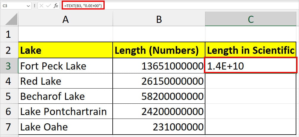
The formula returned 1.4E+10 as an output.
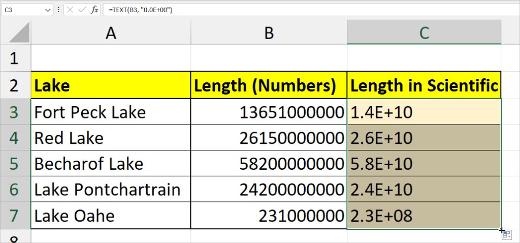
Once you have the result, use Flash-fill to apply the formula for the rest of the columns.
Using VBA Code
For users who find themselves regularly formatting numbers as Scientific Notation, I recommend you run a Macro Code to perform that instead.
Also, although creating Macros is at an advanced level in Excel, do not get intimidated by it. Here, you could just copy-paste the code I’ve compiled in the steps.
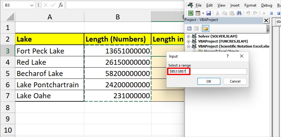
I suggest you perform the given steps in a minimized Excel window as the code will prompt you to select cell ranges with numbers after you run it.
- On your workbook, click the Developer Tab. In case you don’t find it in the ribbon, add them first.
- In Code, select Visual Basic.

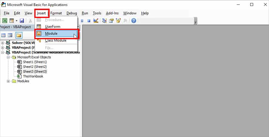
- Head to Insert > Module.
- Copy the code. Then, paste it into your Module.
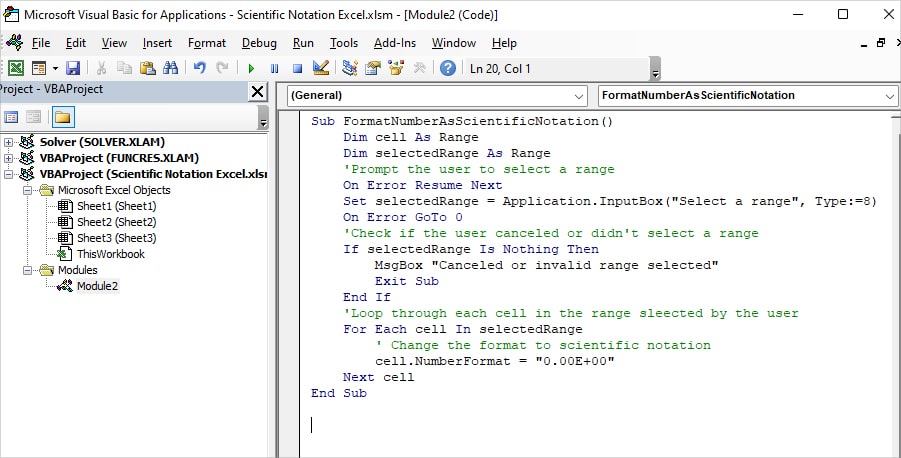
Sub FormatNumberAsScientificNotation()
    Dim cell As Range
    Dim selectedRange As Range
    'Prompt the user to select a range
    On Error Resume Next
    Set selectedRange = Application.InputBox("Select a range", Type:=8)
    On Error GoTo 0
    'Check if the user canceled or didn't select a range
    If selectedRange Is Nothing Then
        MsgBox "Canceled or invalid range selected"
        Exit Sub
    End If
    'Loop through each cell in the range sleected by the user
    For Each cell In selectedRange
        ' Change the format to scientific notation
        cell.NumberFormat = "0.00E+00"
    Next cell
End Sub- Press F5. On the prompt, select Cell range with numbers and hit OK.
Caret Operator
In all the above methods, we learned how to format the number as Scientific Notation, which is in the +E format. But, exponents like 1.78 * 10 ^ (11) is also a Scientific Notation.
Unlike the +E format, there’s no default menu to format numbers as Exponents. So, we will be using the Caret operator and manually input the number.
Using Caret is especially helpful when you have big zeros in your number.
Example:
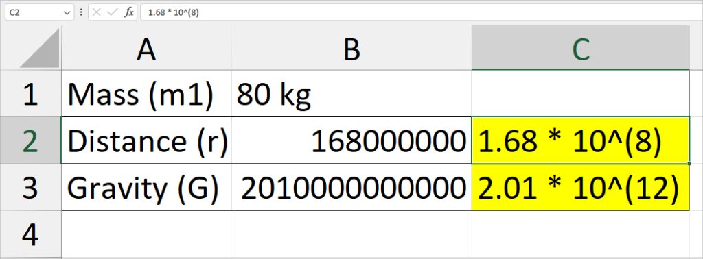
| Number | Scientific Notation |
| 168000000 | 1.68 * 10^(8) |
| 2010000000000 | 2.01 * 10^(12) |
Convert Scientific Notation into Power Base Exponent
For numbers, you must type the power-based scientific expressions yourself. But, if you have +E scientific formats, there’s a formula to convert it into exponents.
We’ll use the LEFT, TEXT, and RIGHT functions nested together.
Formula: =LEFT(TEXT(value, “format value in”), num_chars) & “x10^”&RIGHT(TEXT(value, “format”),3)Example:
Let’s convert the Scientific notation in cell B7. For this, I used the formula as
=LEFT(TEXT(B7,"0.00E+0"),3) &"x10^"&RIGHT(TEXT(B7,"0.00E+0"),3)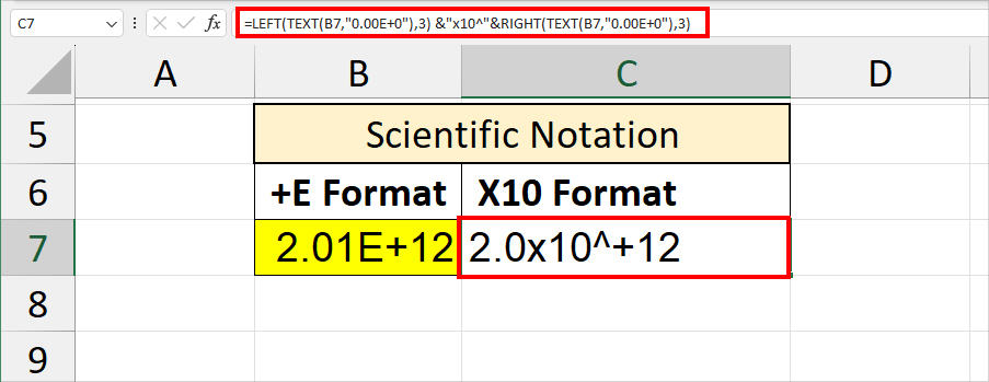
It returned 2.0×10^+12 as output. In the above formula, the LEFT function returns the 3 characters from the left part of 2.01E+12 in “0.00E+0” format which is 2.0. Similarly, the RIGHT function returns 3 characters from the right of 2.01E+12 which is +12.
Finally, the & operator concatenates the result of LEFT, x10 base, and RIGHT functions together.
Stop Numbers for Changing into Scientific Notation
Sometimes, there can be instances when Excel itself applies Scientific Formats to numbers.
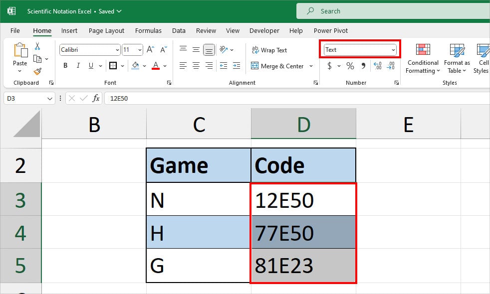
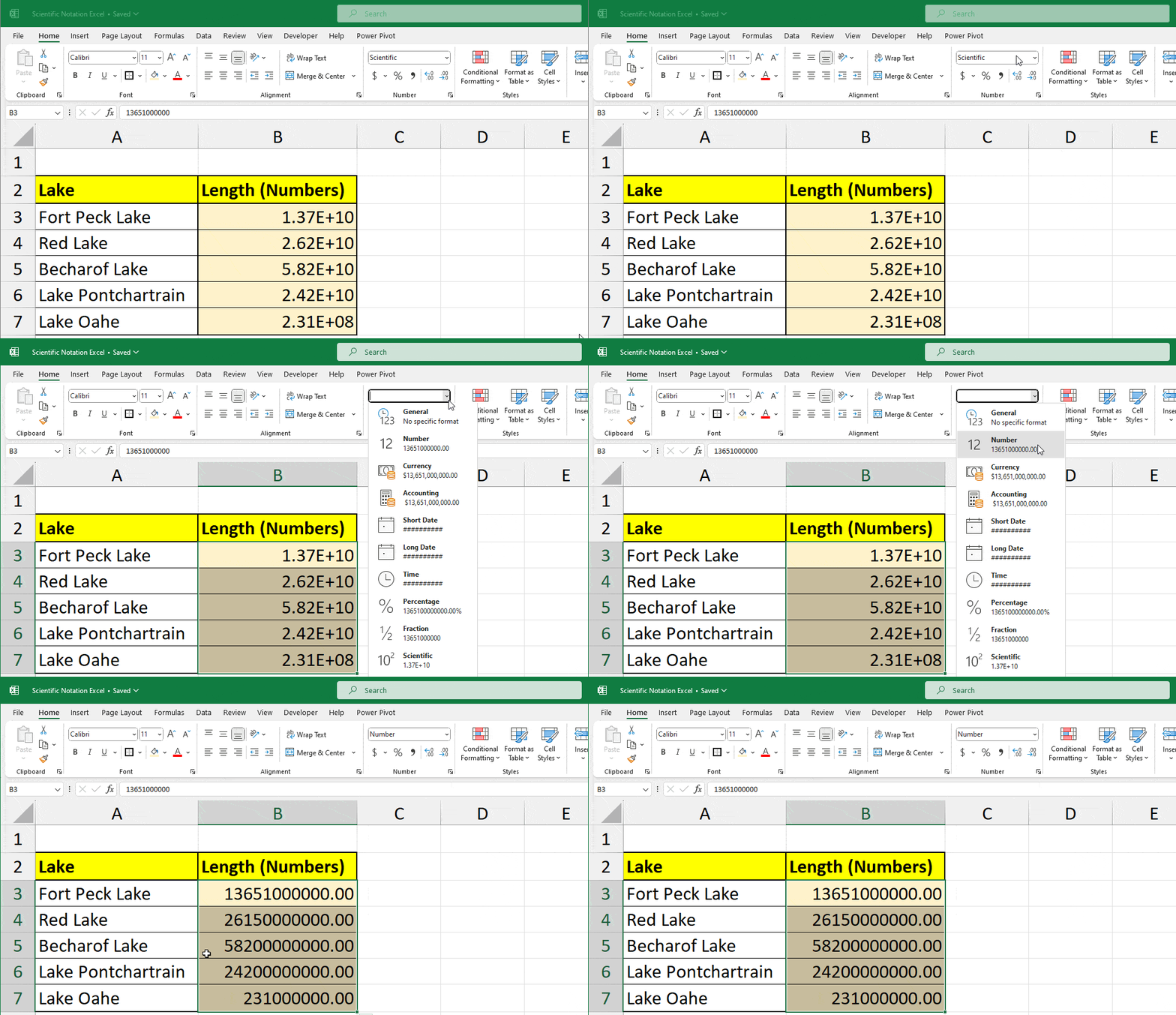
For example, when you type the letter “E” along with numbers like 12E50. Or, when you have big 11+ digits that do not fit in a cell.
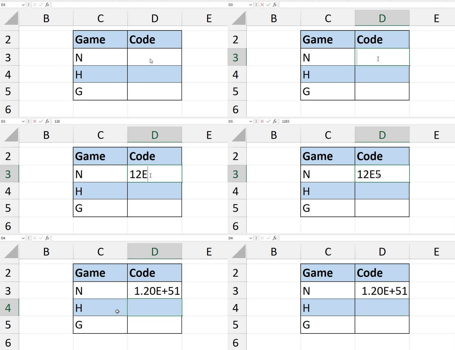
However, if you do not want Excel to automatically change format, we have two methods to stop it.
For numbers with an “E” text string, select an empty cell range and apply Text Formatting. Then, type the values one by one.
Next, for numbers that are in +E due to cell size, select the Cells and set the Format to Number.
For a detailed guide, explore our other article on “How to Stop Excel from Changing.”