How to Remove Text before a Character in Excel

Although the full text could hold a value, in some cases these text can dilute the most important bits for us.

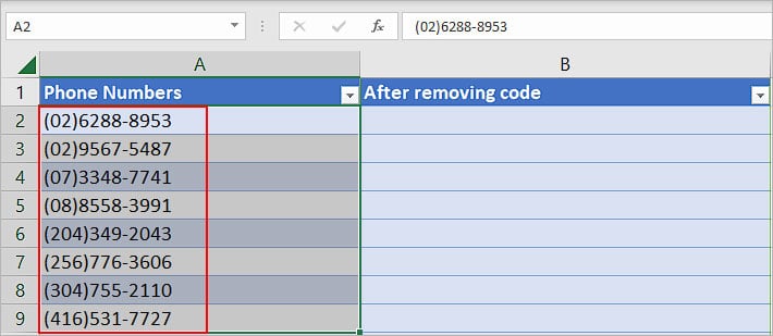
For instance, let’s consider a phone number (02) 6288-8953. Here, instead of the area code we just need the phone number 6288-8953.

If the dataset is small, you could manually edit each cell to remove the area code.
In the case of a larger spreadsheet, there are numerous options and formulas that will get you the desired result without breaking a sweat.

Using Text to Columns

While the Text to Column feature is specifically used to separate texts based on a certain character, you can use it to get rid of certain parts of the text.

Note: This method does not separate the character but removes it completely.

1. Select the cell (s) containing the text.
   
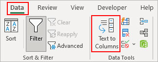
2. Click Text to Columns under the Data tab.
   
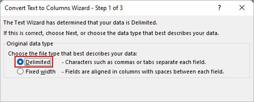
3. On the next prompt, select Delimited and click Next.
   
4. Under the Delimiters section, choose one of the predefined characters. If your text is based on a different delimiter, enable the Other checkbox and enter that character instead. In this case, we want only the part after the round bracket “)”.
   
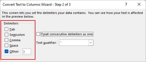
5. Also, enable the Treat consecutive delimiters as one checkbox.
6. On the next prompt, select the Do not import column (skip) option.
   
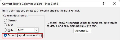
7. Click the Up arrow icon at the end of the Destination field and select where you want the final output.
   
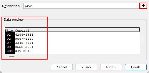
8. Check the Data preview section if you have achieved the desired result. If the output is still not the one you are looking for, click Back and try using a different delimiter.
9. Click Finish.

Using Find and Replace

Typically, we use Find and Replace to search for a particular text and replace it with another text. But we can change it so that everything before the specified character is replaced with a blank character.

1. Copy and paste all the text into a separate worksheet.
2. Then, select the cell (s) with the text and press Ctrl + H.
3. On the Find and Replace window, type the character that separates your text and add an asterisk symbol before it. Here, the symbol is a wild-card character that tells Excel to find everything that occurs before the specified character.
   
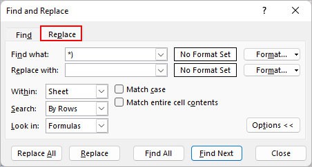
4. Leave the Replace with field empty.
5. Then, click Replace All.

Note: If you have a different character such as a dash, dollar icon, or any other, use them instead of the above round bracket ")".

Using Flash Fill

The Flash Fill is smart enough to detect patterns and autocomplete the remaining selected cells. You can manually fill some cells with the kind of output you want. Then, it should suggest and fill other cells automatically based on the pattern of previously entered values.

1. Enter the text without the character for the first cells or so.
   
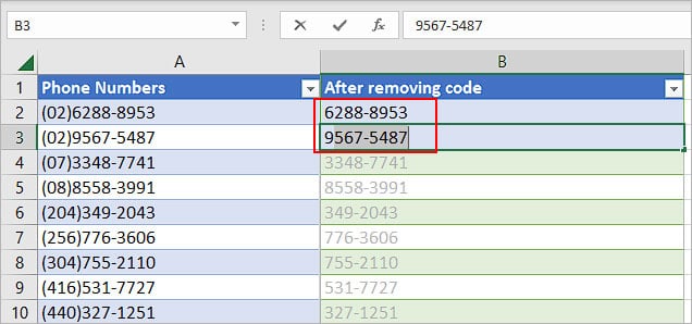
2. Once you start typing the next output in the column, press Enter as soon as Excel suggests and autocompletes other cells.

Using Power Query

Power Query is one of the most powerful tools for importing data from various sources and transforming it using various tools, such as the delimiter. An extra advantage of using it is that you can transform the data multiple times, and easily undo any previous step.

1. Select the cell (s) containing the text.
2. Then, click From Table/Range under the Data tab. You can find the option inside the Get & Transform Data section.
   
3. If you get a Create Table prompt, click OK to convert the selected cells into a table.
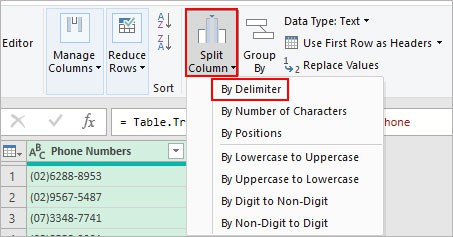
4. Once the Power Query Editor window pops up, click Split Column and select the By Delimiter option.
   
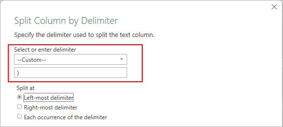
5. Next, select one of the delimiters under Select or enter delimiter section. If your text contains a unique delimiter, choose Custom and enter it.
   
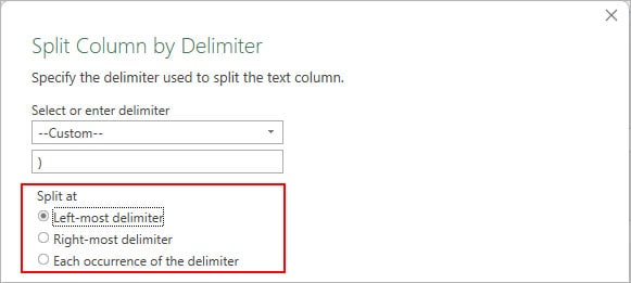
6. If the character appears multiple times in the text, check whether it appears first from the left to right or right to left direction. Then, choose the Left-most delimiter or Right-most delimiter.  In the text (02)6288-8953, the bracket “)” appears first from the left side first. So, we selected left.
   
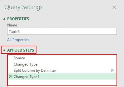
7. Click OK. Or, click the cross icon to delete a step under Applied Steps to revert to the old data.
   
8. After the text is separated into multiple columns, right-click on the unwanted column and click Delete. Or, right-click on the column with the correct output and select Remove Other Columns.
   
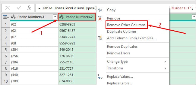
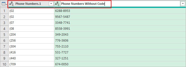
9. Additionally, double-click on the column heading to rename it according to your preferences.
   
10. When done, click Close & Load in the top-left corner to save the final output.
    

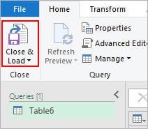
Note: Excel will display the output in a new table. But, you can copy or move it to new location afterwards.

Using TextAfter function

Using the TEXTAFTER function, you can choose to keep only the text that appears after the specified symbol/character. The way it works is by searching for the first occurrence of that character and when found, it ignores all the remaining part before it.

In case, the same character occurs multiple times in the text, you can start the search from the end too.

For instance, if you have a text such as Jack+John+Jr, the function will, by default, start searching from the left and return you John+Jr. 

But, what if you need only the Jr part?

In that case, you can start searching from the end of the text to get Jr.

Syntax: 

=TEXTAFTER(text, delimiter,[instance_num])

Here, 

• text: text you want to split
• delimiter: character that separates the text
• [instance_num]: refers to where the function should start searching for the character. By default, its value is 1, and searches from left to right but stops immediately on the first occurrence. To start searching from the end, use -1.

1. Type =TEXTAFTER( and enter the following arguments.
2. Select a cell (s) containing the text. 
3. Enclose the character inside the quotes.
4. Then, close the bracket to complete the formula and press Enter.
   

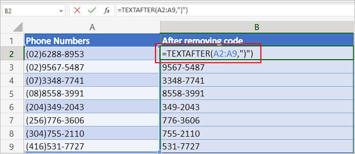
Note: The above function is only available on Excel online and Office 365 as of now.