When transforming a data table or a range into a PivotTable in Excel, you may stumble into the “PivotTable Field Name is Not Valid..” error. This error usually occurs when there’s an empty column header(s) in the source data table. Similarly, you can also get this issue if there are blank or hidden columns.
If you encounter this error, you won’t be able to create a PivotTable. This is because Excel cannot find a name to categorize your data into a Pivot Table.
It’s worth noting that this issue can still occur even if you have already created a PivotTable. If you edit your data source and leave a column blank or hidden, you may still receive this error.
Enter Names for All Column Headers
Pivot Tables are automation tools that provide you with a neatly arranged, summarized form of your data range. If a column header is missing, Excel cannot make such an arrangement.
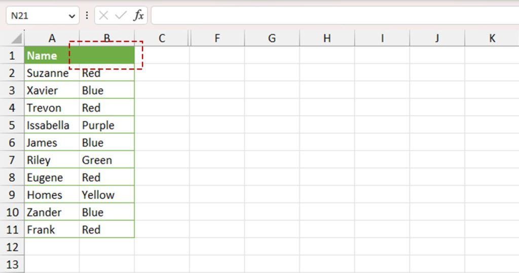
Check your source table and see if any column header is left empty. After filling in the information, try to convert your data to a Pivot Table again and see if the problem persists. If it does, you can move on to the next solution.
Delete Empty Columns
If your data table/range may have an empty column, Excel will fail to categorize the selection to create a Pivot Table. Therefore, the program will trigger this error message as a prompt for you to either fill in data in the empty columns or delete them.
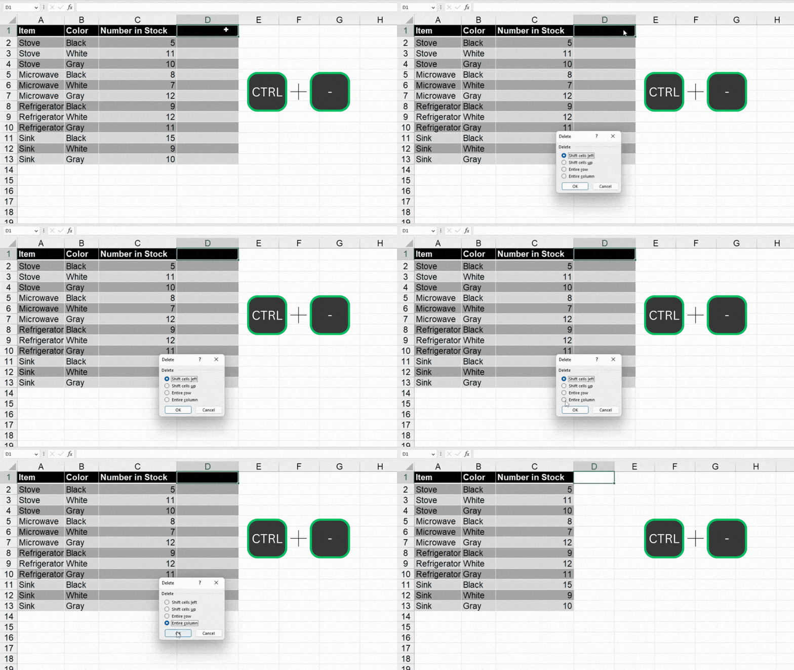
You can choose to enter information in the black column, or simply select it and use the Ctrl + – Excel shortcut to delete the column. If the Delete prompt appears, select Entire Column > OK.
Unhide Columns from Source Data
Hidden columns in the source data range can be equally responsible for this issue in Excel. By now, you may have already understood that columns are integral in creating categories for a Pivot Table. Therefore a hidden column may cause an issue in the order of the Pivot Table.
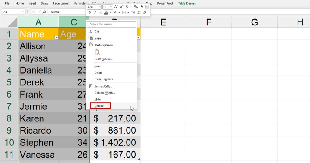
You must unhide the hidden column(s) to create your Pivot Table. If you know where your hidden column is, you can simply select the two adjacent cells, right-click on the header and choose Unhide. If you’re unaware, select the entire range, right-click on the column header, and select Unhide.
Check the Pivot Table Source
If you’re encountering this error after making changes to your worksheet, then you might want to review your selection. You may have made an extra selection that you deleted in the source data range. When trying to refresh the Pivot Table, Excel will prompt this error message.
Check the source and make changes if you must. Firstly, select your Pivot Table and follow these instructions to change the data source for your Pivot Table:
- Head to PivotTable Analyze.
- Select Change Data Source > Change Data Source from the Data section of the ribbon.
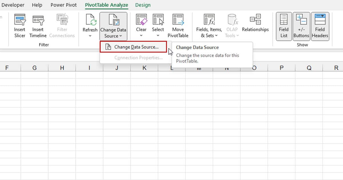
- Check your range. If you see some inconsistencies, select the icon next to the Table/Range section and redo the selection.
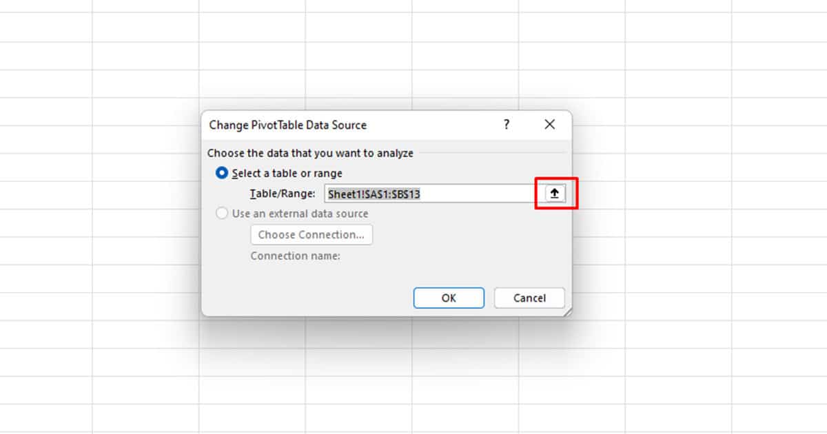
- Click OK.