How to Make a Monthly Attendance Sheet in Excel with Formula

Many users use Excel as a means to store data. If you’re in the HR department of a company, you can use the Excel spreadsheet to keep track of your employee’s working hours, and even create a monthly attendance sheet.

While you can manually create an attendance sheet, you can incorporate formulas within your attendance sheet to make the process more swift. Additionally, using formulas instead of static values will make your data more dynamic.

Step 1: Enter the Month and Dates

We will first have to specify which month our data was recorded.

As an example, let’s assume our sheet is for the month of January. In cell A1, I entered Month and merged it with cell A2. Then, as January has 31 days, I merged 31 cells from range C1:AG and entered January.

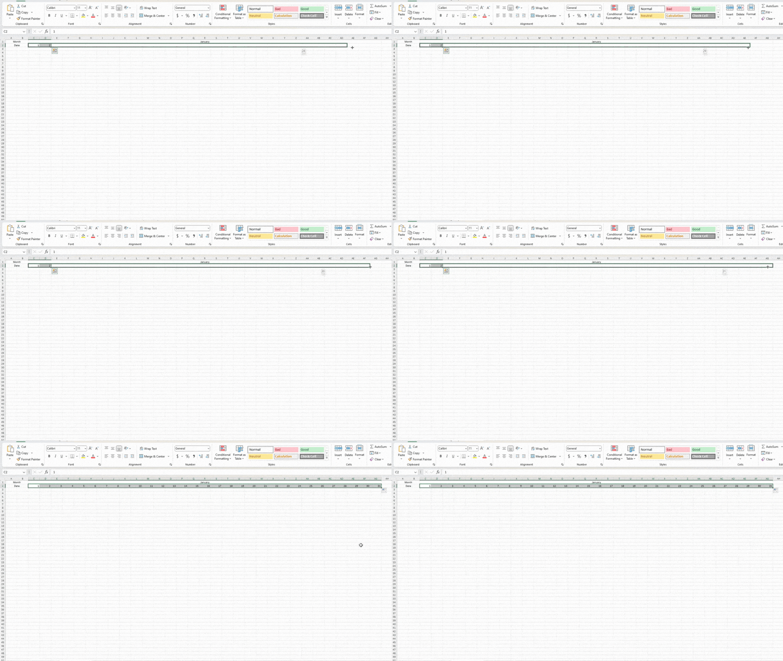
Under Month, I entered Date in cell A2 and merged it with B2. Then, I entered 1 and 2 on cells C2 and D2 respectively. To automatically fill in the rest of the numbers, I selected cells C2 and D2 and placed my cursor on the bottom-right corner of D2. After the cursor changed to a “+”, I dragged it to cell AG. This process is also called Flash Fill.

Step 2: Enter the Symbol Number and Name

After entering the Month name and dates, we can begin entering the basic information, the symbol number the names of your employees. You can manually enter these values, but if you already have this information on another sheet or workbook, you can use a formula to reference those values to the current sheet.

In our example sheet, we have the names of our employee and their IDs in the EmployeeDetails sheet from range A1:B12. Let’s use 3D referencing to reference these values to our monthly attendance sheet.

In cell A3, I entered the following formula:

=EmployeeDetails!A1:B12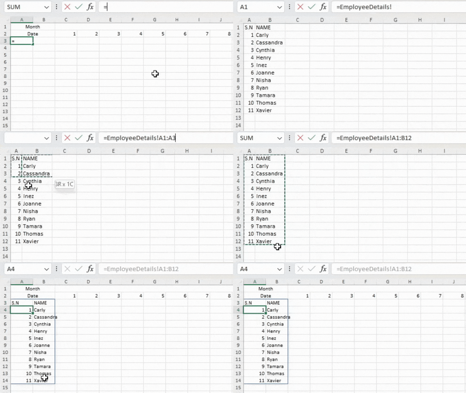

Step 3: Add Days of the Week

We can now add the days of the week to our attendance sheet.

In cell C3, I entered the acronym for Sunday, “Sun”. We can again use Flash Fill to automatically fill in the days to the rest of the cells.

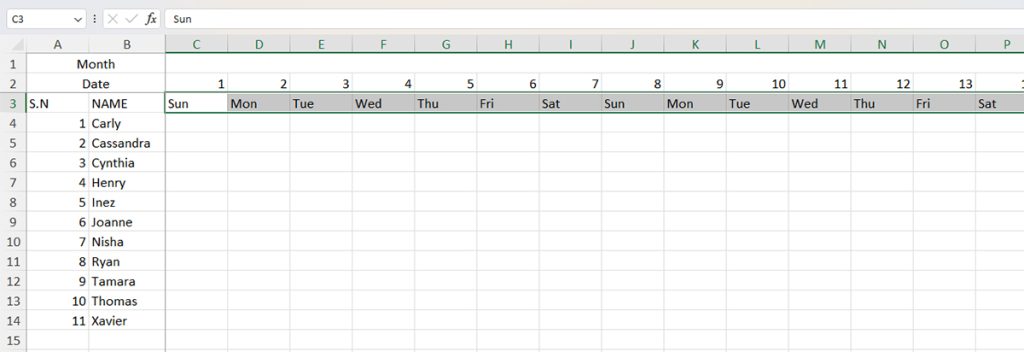
Select cell C3. Then, place your cursor on the bottom-right corner of the cell. Once the cursor shifts to a +, drag it to cell AG. The days of the week will be pasted in the same format. As you can see, I used an acronym for Sunday. Excel pasted the rest of the days following the same acronym.

Step 4: Enter Attendance

You can then enter the attendance in range C4:AG14.

While entering the values for present, and absent, make sure you’re consistent. In our sheet, I used “A” for Absent and “P” for Present. You can use similar characters to represent present and absent in your attendance sheet.

Step 5: Calculate the Total Working Days

Let’s now count the total number of working days in the month of January.

I have left the columns that represent off-days blank. Using this information, I can use the COUNTA function to only count cells with the text, “A” or “P” in them.

Here is the formula to count the total working days using the COUNTA function:

=COUNTA(C4:AG4)

As this data is common between all fields, I merged the cells till cell AH14.

Step 6: Calculate the Total Days Present

We can use the COUNTIF function to calculate the total number of present days of an employee.

For COUNTIF to calculate accurately, you must make sure to use the same value to mark a person present. For example, you cannot use both “P” and “Present” in your attendance sheet.

Here is the formula we used with the COUNTIF function to compute the total number of present days:

=COUNTIF(D4:AG4,"P")

Step 7: Calculate the Total Days Absent

We will again be using the COUNTIF function to calculate the total number of days an employee was absent in the month of January.

Here is how we constructed the COUNTIF formula to count the total number of days absent:

=COUNTIF(D4:AG4,“A”)

Use Flash Fill to fill in the rest of the value.

Optional: Apply Formatting

Although our attendance sheet is complete, it still looks quite incomplete. If you like making your document look more presentable, you can use different formatting tools in Excel to beautify your spreadsheet.

Change Text Alignment

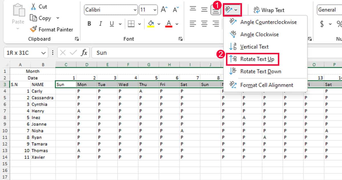
For this sheet, I want to rotate the data in range C3:AG3, containing the names of the day, up. Here is how you can change the text alignment to rotate your data upwards:

1. Select your data range.
2. Head to the Home tab.
3. From the Alignment section, select Orientation.
4. Choose Rotate Text Up.
   

Use Conditional Formatting

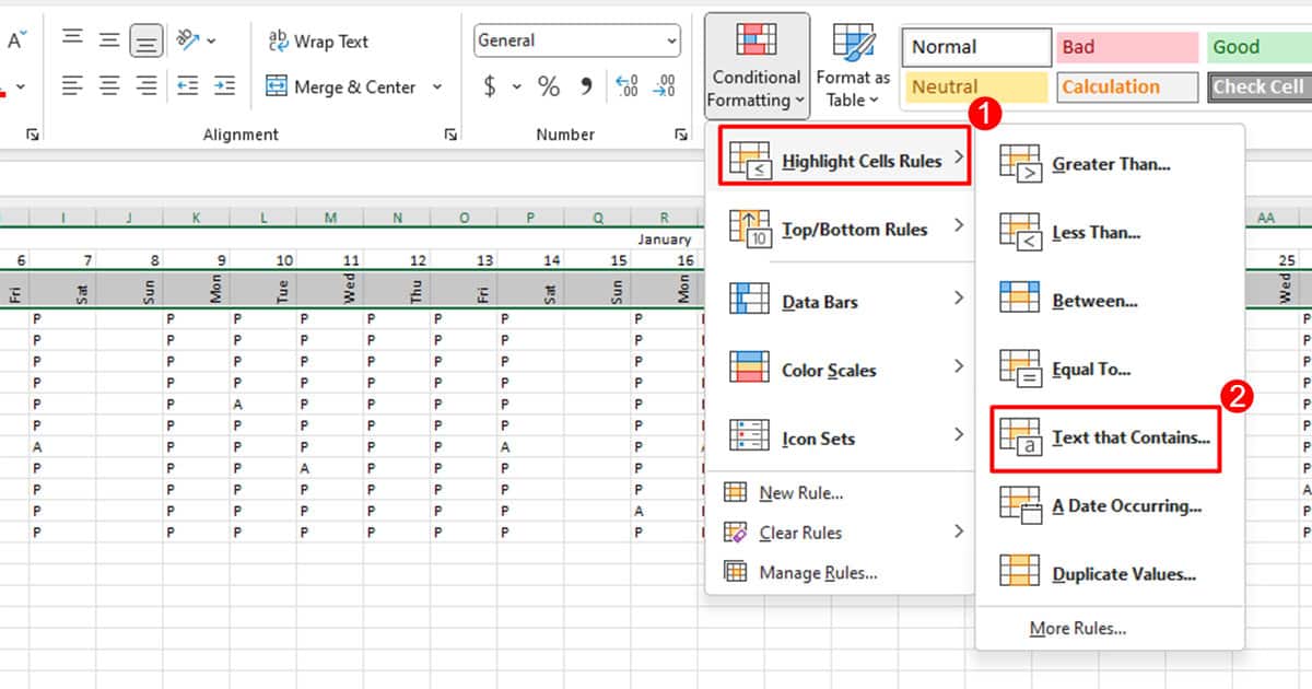
You can use conditional formatting to highlight cells that contain any information you wish to draw attention to. For an attendance sheet, you can use conditional formatting to highlight the off day of the week. In our sheet, the off day is Sunday. Here is how we set the rule for conditional formatting to highlight the cell containing “Sun”.

1. Select your data range.
2. From the Home tab, select Conditional Formatting from the Styles section.
3. Choose Highlight Cells Rules > Text that Contains…
   
4. Under Format cells that contain the text, I entered Sun.
   
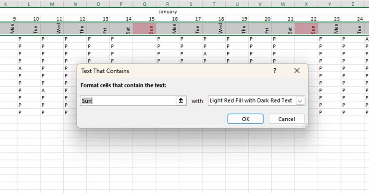
5. In the next field, use the drop-down to select a formatting option.
6. Click OK.