How to Merge or Combine Tables in Excel

If you’ve imported or created multiple tables in Excel sheets, you may find the need to merge them together into one. Having all data in a single table is simply so convenient to analyze information and input formulas. 

In most cases, some users would copy Table 2 and paste them into the adjacent cells of Table 1 to combine them together. This workaround, however, is ineffective if your table is extremely large or does not correspond.

So, the most easiest yet effective way to merge any tables is using the VSTACK function. With this function, you can combine numerous tables within sheets, from different sheets, or separate workbooks. However, for users who do not have access to this function, you could use VLOOKUP, Power Query, or Consolidate tools. 

Using VSTACK Function

Excel’s VSTACK function combines the number of vertical arrays into a single array. This function is perfect for merging tables within the same sheet, different sheets, and different workbooks. 

Syntax: =VSTACK(array1,{array2],..)

As this function is relatively new, you must open Excel on Office 365 or the Web version to use it. 

Case 1: Merge Tables in the Same Sheet

In the given example, we are combining three tables into a single one within the same sheet. For this, I entered the formula as

=VSTACK(A1:B6, A9:B13, A16:B20)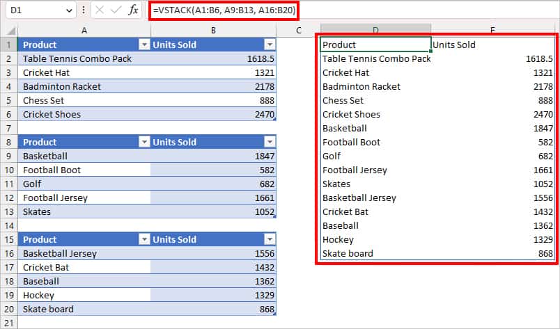

In the above formula, A1:B6 is Table 1, A9:B13 is Table 2, and A16:B20 is Table 3. While selecting the values, make sure to skip the table heading for Tables 2 and 3. 

Case 2: Merge Tables in Different Sheets

VSTACK function also makes it easier to combine tables from different sheets of the same workbook. 

Suppose, you need to integrate tables from Sunday, Monday, and Tuesday sheets. For this, we entered the given formula in the Cell A1 of a new sheet.

=VSTACK(Table_1[#All], Table_2, Table_3)

Note that before entering the formula, we first renamed all Tables from the Table Design tab. Now, let’s see how we took the array reference in the formula. 

• Firstly, enter =VSTACK( in an empty cell. 
• Then, go to Sunday sheet and select the Table reference i.e. A1:B6. Put a comma and do the same for other sheets. When done, close the Parenthesis and press enter.

In the above example, we just took three sheets as a reference. But, you can take reference from as many references as you want.

Case 3: Merge Tables in Different Workbooks

Say, you have tables in different workbooks and wish to integrate them into one. For this, we will use a similar formula as above. However, it is only effective if you have a corresponding table. If it isn’t, the formula will result in Spill 0 where there is no value. 

As a reference, we will combine tables from Merge Tables and Table workbook. To do so, we first opened the workbook in side by side view. Then, we entered the formula below.

=VSTACK(Table_1[#All], Table.xlsx!Table_2[#Data])

Let’s see how we added this formula. 

• Firstly, type in =VSTACK( on an empty cell of your current sheet. Then, select the table from that sheet.
• Now, enter a comma in the formula. Go to another open workbook and select the table. Close the Parenthesis and hit Enter.

Using Power Query

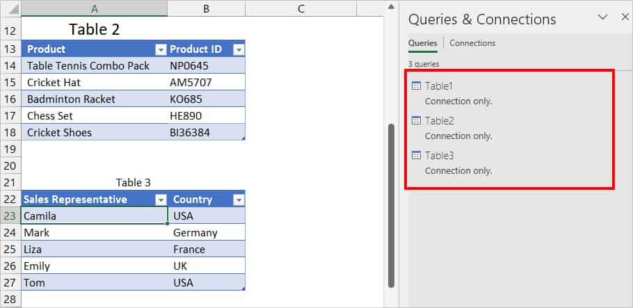
In the above method, we merged two tables having identical data value with the VSTACK function. But, there can be instances when the table you wish to combine does not correspond with other tables like in the image below.

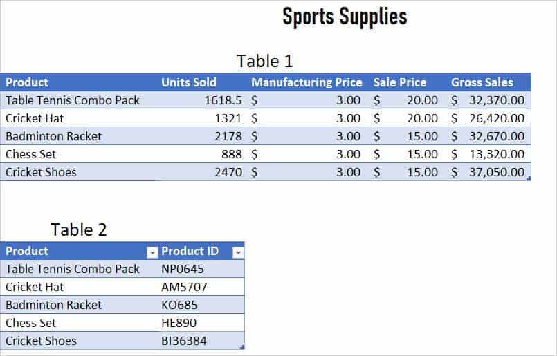
Suppose, you need to consolidate these two tables into one. For this, we will use the Power Query tool. Here, we will create a connection in all tables and merge them. To do so, your data must be in Table Format.

Step 1: Create a Connection in Queries

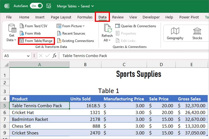
1. Click on any cell of Table 1.
2. On Data tab, click on From Table/Range.
   
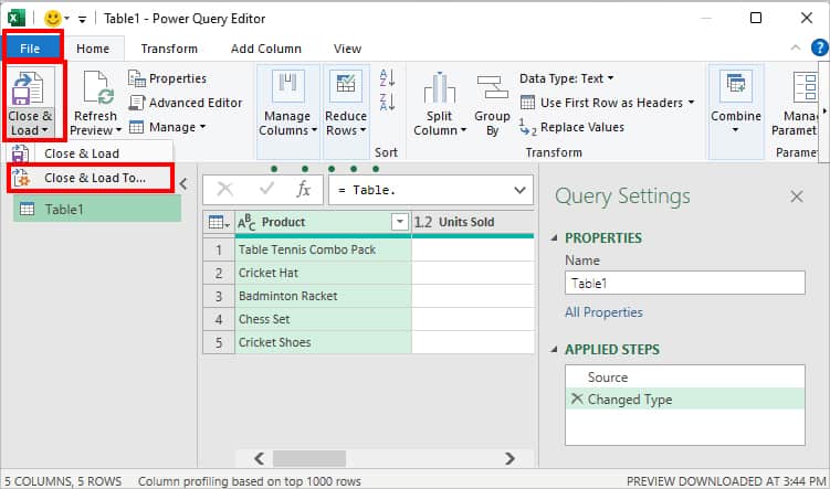
3. On Power Query Editor window, go to File Tab. Click on Close & Load > Close & Load To.
   
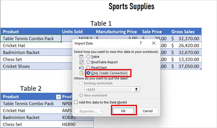
4. Under Select how you want to view this data in your workbook, pick Only Create Connection. Then, hit OK. 
   
5. Again, repeat Steps 1 to 4 to create Connections for the rest of the tables too. On the Queries & Connections menu, you should see all the tables. 
   

Step 2: Merge Queries

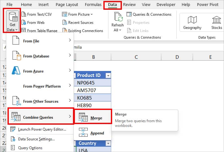
1. On your worksheet, go to Data Tab.
2. On Get & Transform Data group, click on Get Data.
3. Hover Over Combine Queries > Merge.
   
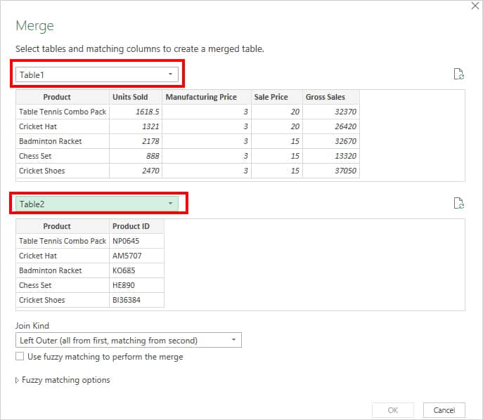
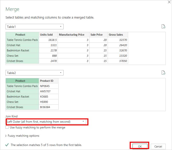
4. A merge window will appear on your screen. Expand the drop-down menu and select a Table. Again, second select Table to merge.
   
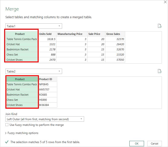
5. Now, Select the identical columns on your table.
   
6. Under Join Kind, leave the option to Left Outer(all from first, matching from second). Click OK.
   

Step 3: Close & Load Table

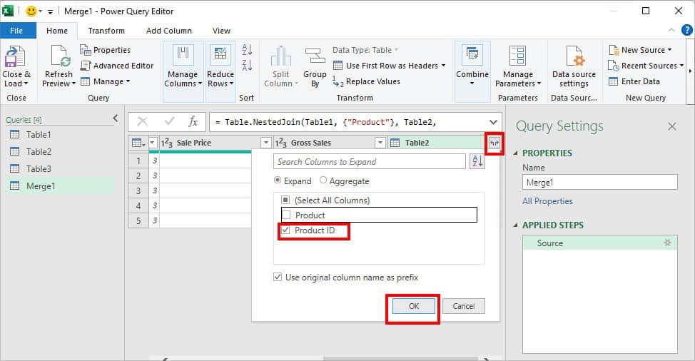
1. On Power Query Editor Tool, hover over the Merged Table and click on Expand Icon.
2. Only tick on the Column you want to expand and hit OK. 
   
3. If needed, swap Column position.
4. From File Tab, click on Close & Load > Close & Load. 
   
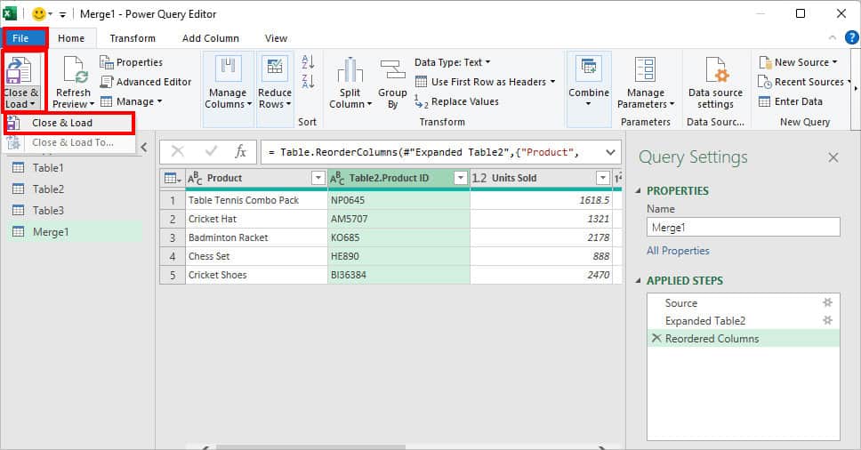
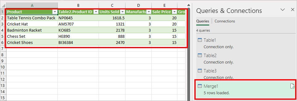
5. The merged table will appear on the new sheet.
   

Using VLOOKUP Function

Another way to join several tables into a single is by using the VLOOKUP function. I recommend you use this method if you are sharing your workbook with older Excel version users.

Excel’s VLOOKUP function is mostly used to locate the values in the table. You could even join the tables that do not correspond with each other. But, the tables must have at least one column in common for this function to work.

Syntax: VLOOKUP(lookup_value, table_array, col_index_num, [range_lookup])

• Lookup_value: value to look for in the First column of Table
• Table_array: range in a table VLOOKUP looks for the lookup_value
• Col_index_num: Values to return from column number
• [range_lookup]: logical value which is either Approximate match or Exact match. (Optional)
  • Approximate match -1/TRUE searches the nearest value if VLOOKUP does not find the exact value. 
  • Exact match – 0/FALSE looks for the specified value/range in the column.

Let’s suppose, we need to merge the given two tables using VLOOKUP. For this, enter the formula as

=VLOOKUP([@Product],Table2, 2, FALSE)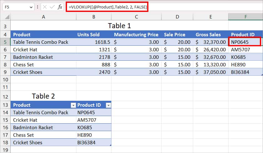

In the above formula, VLOOKUP will return the value in the same row as [@Product] which is the first column of Table 1. By passing, the FALSE range_lookup argument, it will look for the precise value in Table 2’s second column which is the Product ID. As a result, you’ll get all Product ID values in Table 1.

Using Consolidate Tool

Excel’s Consolidate Tool returns the summed-up value of ranges within the same sheet or different sheets. Meaning, it integrates all duplicate data of a table and consolidates the output in a single range. Use this method if you wish to extract only unique values from a table.

1. Create a New sheet in your workbook.
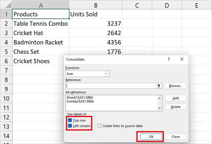
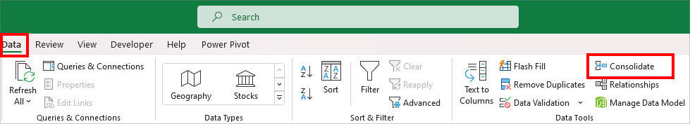
2. Head to Data Tab and click on Consolidate.
   
3. Click the Collapse Icon on Reference. Select the Table Reference. 
4. Next to All References, click Add.
   
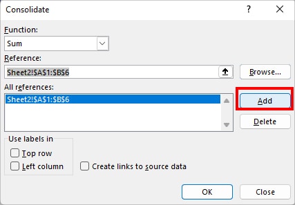
5. Repeat step 3 & 4 for other tables. 
6. Under Use labels in, tick Top row and Left column box. Click OK.