In Excel, Lookup tables are widely used in huge databases as a reference to extract the value from. You could be using the Lookup table to evaluate Sales Sheets, remark Marksheets, Count Numeric Inequalities, and so on.
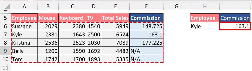
Lookup Tables are simply your existing data table which you use to look for a value. Suppose, if I need to return the Commission rate of Employee Kyle, I will look for the value in a table ranging from A6 through F10. So, in short, A6:F10 is my Lookup Table.
If you have large records, it is impossible to skim through the lookup table manually and locate the exact value. To ease your work, Excel has various lookup and reference functions that’ll help you to search the value horizontally, vertically, or both ways.
If you’re ready, let’s get started and make the best use of lookup tables with these functions.
How to Use Lookup Tables With Examples
In the given examples, we have mainly discussed the most common and extensively used lookup functions such as VLOOKUP, INDEX and MATCH, HLOOKUP, XLOOKUP, and OFFSET.
Using VLOOKUP Function
Among the lookup and reference functions, VLOOKUP is the mostly used function in Excel. It is mainly because it is available in all Excel versions ranging from 2010 to the latest 365 versions. You can use the VLOOKUP function to look for a specific value in a column within a table range.
Syntax: VLOOKUP(lookup_value, table_array, col_index_num, [range_lookup])- lookup_value: Value you want to search
- table array: A table range to look for the look_up value
- col_index_num: Column number that has the value to return to
- [range_lookup]: Boolean to specify whether to return an exact match or approximate value.
- 1(TRUE): Return approximate value
- 0(FALSE): Return exact value
Example: Let’s use the VLOOKUP Function to return the value from a Lookup table. Suppose, we want to return the Commission of Tom in cell I6. For this, we entered the formula as
=VLOOKUP(H6, A6:F10, 6, 0)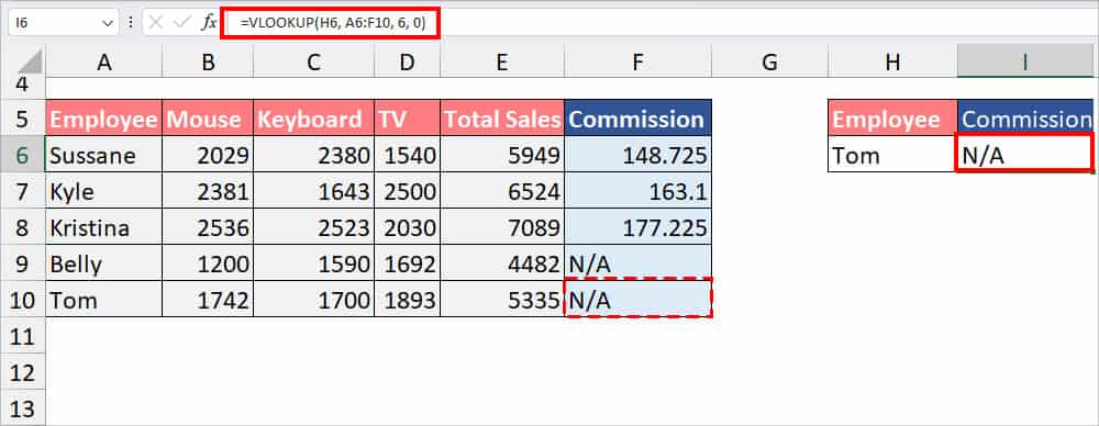
In the formula, cell H6 which contains Tom will be our lookup value. Similarly, our lookup table range is A6 through F10. Since the Commission column is in Column F, we’ve entered the 6 as a Column Index. We’ve specified the formula to return the exact match with the 0 boolean logic in the formula. As a result, it returned the commission of Tom which is N/A.
Using INDEX and MATCH Function
While INDEX and MATCH functions are Excel’s two separate lookup and reference functions, they are mainly used nested together. By nesting the MATCH function inside the INDEX function, you could even perform powerful lookups.
You could use this function as an alternative to the VLOOKUP function if your lookup value isn’t in column 1. In INDEX and MATCH, the lookup value could be in any column.
| Function | Syntax | Function Arguments | Description |
| INDEX | INDEX(array, row_num, [column_num] | array: Cell range that contains your value row number: Row index that has your value [Column number]: Column Index to return your value from | Returns the specified item from a table. |
| MATCH | MATCH(lookup_value, lookup_array, [match_type]) | lookup_value: value you want to search and return. lookup_array: Array that contains the lookup_value. [match_type]: Specify the behavior to lookup for a value 1: Returns the largest value 0: Returns the exact value -1: Returns the smallest value | Returns the position of the lookup value in the range. |
Example: Let’s suppose, we need to return the Keyboard Sales of employee Tom. With the INDEX and MATCH functions nested together, our formula would be.
=INDEX(C2:C6, MATCH(H3, A2:A6,0))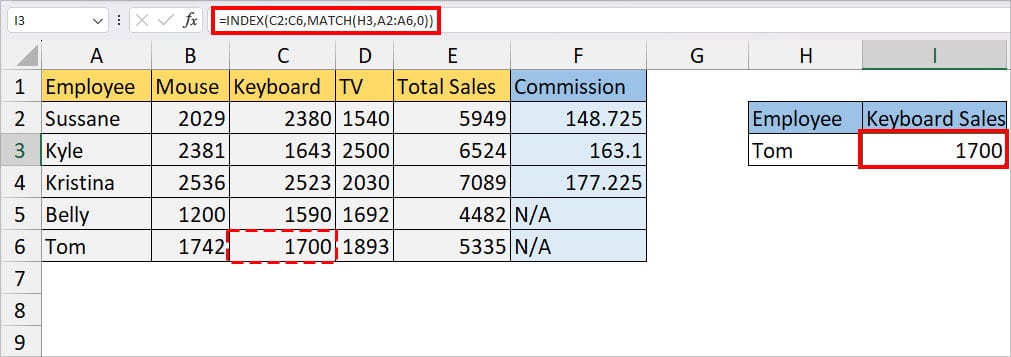
In the formula, firstly, MATCH(H3, A2:A6, 0) formula returns the exact position of our lookup value “Tom” from the cell range A2:A6. It returned 5. Then, the INDEX(C2:C6, MATCH(H3, A2:A6,0)) formula returns the value of the 5th position from cell range C2:C6. Thus, it returned 1700.
Using HLOOKUP Function
The VLOOKUP function is used to search for values in the vertical array. But, if you need to look for values in a horizontal array, there’s a HLOOKUP function.
Excel’s HLOOKUP function returns the lookup value from the specified row index within a certain range.
Syntax: HLOOKUP(lookup_value, table_array, row_index_num, [range_lookup])- lookup_value: the value you want to search in the row
- table_array: range of table to search the lookup_value
- row_index_num: row number that contains the value you want to return
- [range_lookup]: Boolean logic with TRUE or FALSE.
- TRUE: Return the nearest match when the value is not found.
- FALSE: Return exact match. If there are no values, it’ll return a #N/A error.
Example: Suppose, we have a Lookup table with Employee, Mouse, Keyboard, TV, Total Sales, and Commission. We want to find out the Total Sales of an employee named Belly. For this, we will enter the HLOOKUP formula as
=HLOOKUP("Total Sales", A1:F6, 5, FALSE)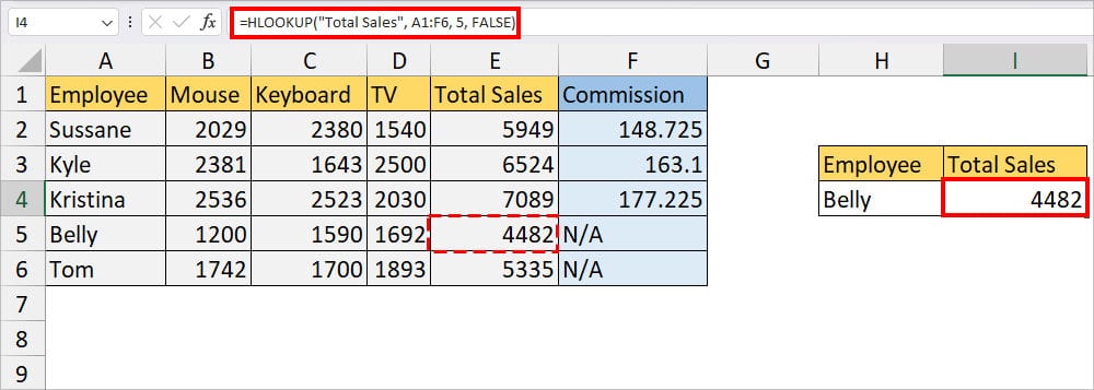
In the formula, our Lookup value is “Total Sales” and the table range is A1:F6. Since the data of Belly is in the 5th row, 5 will be our Row Index. As we’ve specified FALSE, it will return an exact match or #N/A if the value is not found. The formula returned 4482.
Using XLOOKUP Function
Next, we have XLOOKUP Function, which you could also use as an alternative to the VLOOKUP and HLOOKUP functions. This is because the XLOOKUP function is more advanced, works both horizontally and vertically, and can return an array from the lookup table. So, if you need to extract multiple items based on a single value, use this function.
Since the XLOOKUP function is new, it is available only in Office 365 and Excel Web versions as of now. If you have access to this function, check out the example to use this function.
Syntax: XLOOKUP(lookup_value, lookup_array, return_array, [if_not_found], [match_mode], [search_mode])- lookup_value: Item you want to look
- lookup_array: Range to search lookup item
- return_array: Cell range that has the value to return
- [if_not_found]: Return value if the array is empty
- [match_mode]: Boolean logic to specify the formula to return when the value is not found.
- 0: Exact Match
- -1: Closest Smaller Item
- 1: Closest Larger Item
- 2: Wildcard character
- [search_mode]: Specify search mode
- 1: Look for values from the first item.
- -1: Search values from the last item.
- 2: Search values in ascending order.
- -2: Look for values in descending order.
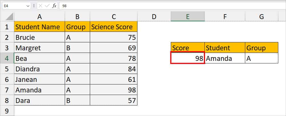
Example: We have data of Student Names, Groups, and Science Scores in our worksheet. Let’s suppose, we want to return the student name and group based on the score. So, here, we need two items to extract.
For this, enter the formula as
=XLOOKUP(E4, C2:C8, A2:B8, "No Value", 0)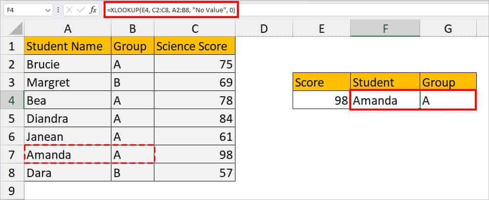
In the formula, our lookup value is in cell E4(98) and the value lies in the C2:C8 array. To extract the Name and group, our return array is cell ranges from A2 through B8. We have specified “No Value” to return if the value is not found within the ranges. To return the exact match, we entered 0 as boolean logic.
Thus, the formula returned Amanda and A as a result.
Using OFFSET Function
Excel’s OFFSET function is another lookup function that returns the item from the reference point of the number of rows and columns you specify. Use this function when you have two lookup tables to look for the value.
Syntax: OFFSET(reference, rows, cols, [height], [width])- reference: Cell range that’ll be your reference point. It will be the base for the rows and column numbers you insert to return in the formula.
- rows: Number of rows your value is located in.
- Positive number: Enter a positive number if your reference point is above the data table.
- Negative number: Enter a negative number if your reference point is below the data table.
- cols: Number of columns that contains the value to return.
- Positive Number: Use the positive number if you want to return the value to the right of the reference point.
- Negative Number: Enter a negative number when you want to return the value to the left of the reference point.
- [height]: number of rows if you want to return an array.
- [width]: number of columns if you wish to return an array.
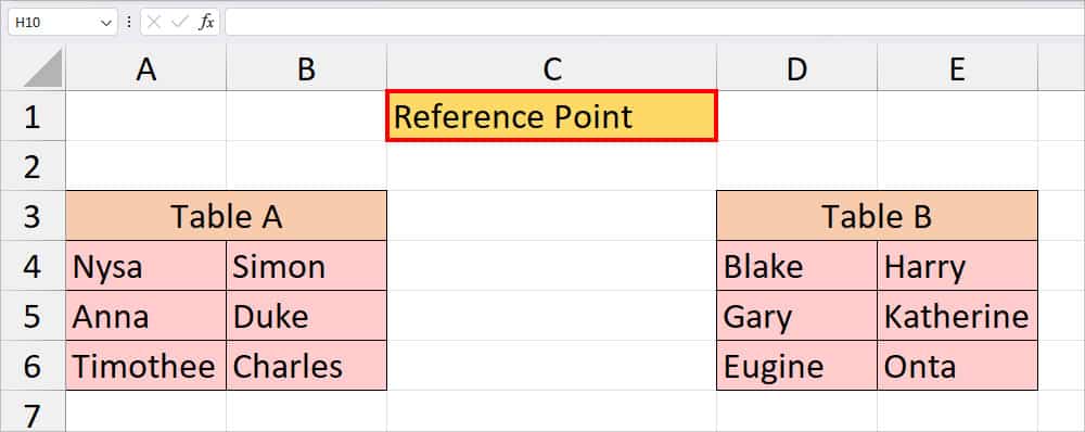
Example: Suppose, we have Table A from cell range A4: B6. Similarly, we have Table B from D4:E6. Firstly, we’ve created a Reference Point in cell $C$1. So, the reference point will be the factor to return the columns and rows from the lookup table.
Suppose, we want to return Nysa from Table A and Gary from Table B.
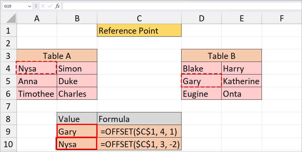
| Value | Formula | Description |
| Gary | =OFFSET($C$1, 4, 1) | The value Gary is in cell D5 of Table B. So, we’ve passed down the argument to return the 4th row and 1st column from the right of reference point. |
| Nysa | =OFFSET($C$1, 3, -2) | The value Nysa is in cell A4 of Table A. So, we’ve passed down the argument to return the 3rd row and 2nd column from the left of the reference point. |
How to Make Dynamic Use of Lookup Tables?
When you solely use the lookup functions, it returns only the specified item or an array. But, let’s make it a more dynamic use of such functions. You would rather switch values for automated lookups than change the arguments in the formula, right?
For this, we will create a drop-down list using the Data Validation tool. After you add a drop-down list, you can simply change the lookup values in the list to return that item.
You could use this trick for all of the lookup functions we mentioned above. But, as an example, we will create a drop-down list for the XLOOKUP function in the given steps.
- On your sheet, select the Cell with lookup value.
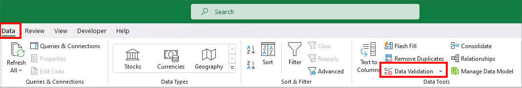
- Go to Data Tab and click on Data Validation from the Data Tools group.
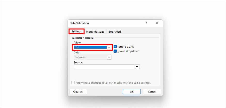
- On the Data Validation window, stay on the Settings tab. Below Allow, pick List.
- On Source, select the Cell ranges of lookup value using the collapse icon and click OK.
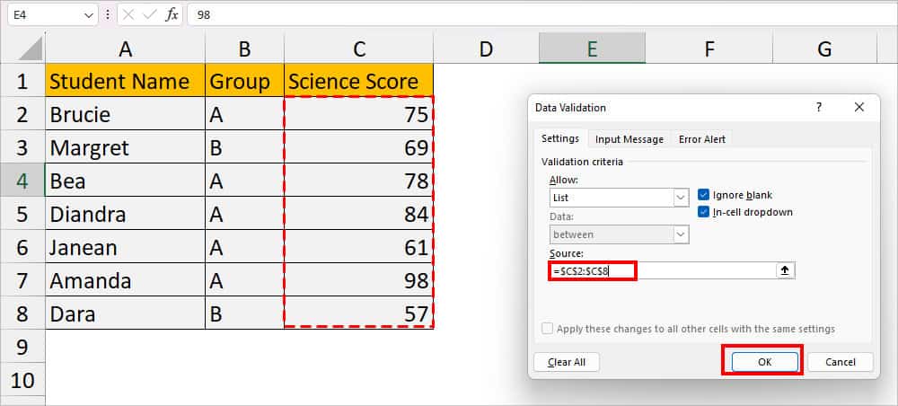
- Now, if I choose a different lookup value in Score, the formula will update accordingly in the result cell.