During Excel Calculations, you may get a different type of cell error message when the formula is incorrect. But, with Excel’s ISERROR function, you can test whether the expression would return an error or not, beforehand.
If you want, you could also use the ISERROR to replace the errors with a specific message in a cell. For example, #N/A with “Not Value Found.”
KEY TAKEAWAYS
- ISERROR function tests whether a cell or expression has #NUM!, #NULL!, #CALC!, #VALUE!, #DIV/0!, #SPILL!, #N/A errors or not.
- The function returns a Boolean value like TRUE or FALSE.
- ISERROR and ISERR functions are different.
- You can use ISERROR to replace the boolean value with the message, return value if error, and count the number of error cells.
- IFERROR function is an alternative to IF and ISERROR nested functions.
What is ISERROR Function in Excel?
Excel’s ISERROR function returns a TRUE or FALSE when there is an error in the tested value. If your cell contains #NUM!, #NULL!, #CALC!, #VALUE!, #DIV/0!, #SPILL!, #N/A, it’ll return TRUE. Likewise, for cells with no errors, the ISERROR returns FALSE.
The ISERROR function only takes up a value as an argument. In the formula, the value can be any expression, text, number, or cell reference you want to test.
Syntax: ISERROR(value)Differences Between ISERR and ISERROR
Mind you, just like the “ISERROR,” there’s another function named “ISERR” that checks whether a value has an error or not. The ISERR function returns TRUE for error cells and FALSE when there’s no any. Since the functionality is pretty similar, most users think these functions are the SAME. But, they are not!
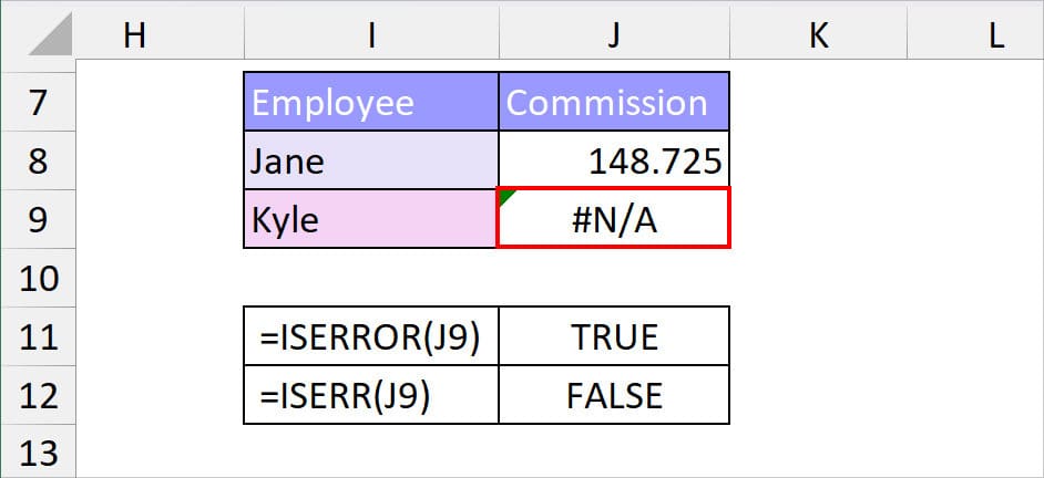
Well, the major difference between them is the #N/A error. The ISERR function does not identify the #N/A as an error. Due to this, even if the cell contains a #N/A, it results in FALSE.
On the other hand, ISERROR takes the #N/A as an error and returns TRUE as you can see in the picture.
As long as your data does not have a #N/A error, it shouldn’t matter whether you use ISERR or ISERROR. But, I do recommend you go for the ISERROR to avoid incorrect results.
Basic Example of ISERROR Function
Here’re very basic examples of the ISERROR function. We will test if the cells contain or the expression would result in an error or not.
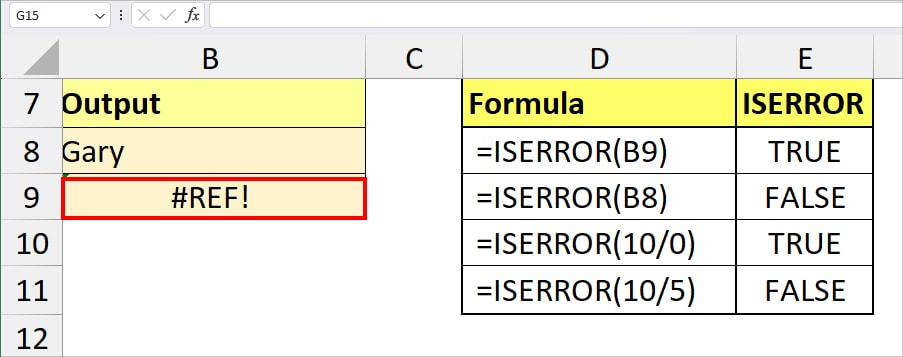
| Value | Formula | Output | Description |
| B9 | =ISERROR(B9) | TRUE | ISERROR returned true because there was a #REF! Error in the cell. |
| B8 | =ISERROR(B8) | FALSE | Cell B8 has a value and no errors. |
| 10/0 | =ISERROR(10/0) | TRUE | Any number divided by 0, returns #DIV/0! error. Thus, the ISERROR returned TRUE. |
| 10/5 | =ISERROR(10/5) | FALSE | This time the number 10 is divisible by 5 and returns 2 as a result. Therefore, the ISERROR returned FALSE. |
Applications of ISERROR Function in Excel
From the above example, we learned how to use the ISERROR function solely to test the error. But, in actual practical life, ISERROR has much more significant applications than that. You could nest this function with others for the maximum benefit.
Switch Boolean Value with Message
If you’re familiar with Excel’s IF function, you might know that the IF function returns only Value if true and Value if false results for a logical test. To return a different item, you can use the ISERROR and IF function nested together.
Example: Here, I have a Table with Product ID, Products, Quantity, Total Price, and Unit Price. Suppose, I want to find out the Unit Price by dividing the Total Price and Quantity.
For this, I entered the IF and ISERROR formula as below and extended the Flash-Fill.
=IF(ISERROR(D2/C2), "No Quantity", D2/C2)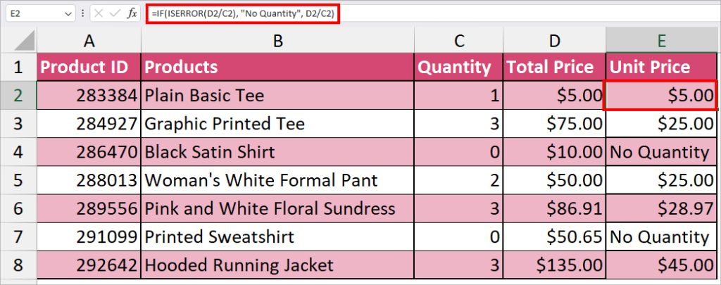
In the above formula, firstly, the ISERROR checks whether D2/C2 contains an error or not. It returned FALSE. Then, the IF function takes the ISERROR(D2/C2) as a logical test, “No Quantity” as Value if True, and D2/C2 as Value if False. As a result, we got 5 in cell E2.
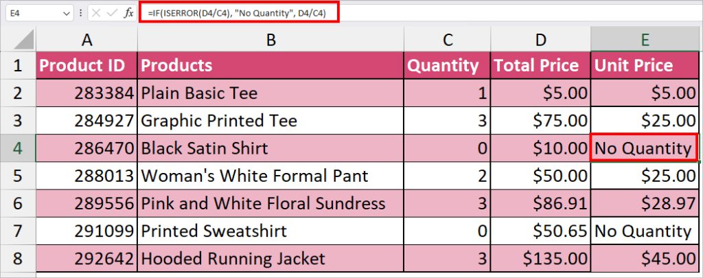
But, if you see in cell E4, the formula returned No Quantity. This is because the D4/C4 (10/0), would result in #DIV/0! Error.
Return Value If Error
While using the VLOOKUP functions in Excel, especially with the FALSE argument, you’ll receive a #N/A error when there’s no value to return to. If you have a workbook full of #N/A in cells, it can look very messy and unprofessional.
But, what if you can replace the error with something like “No Value” or “No Value Found?” Such phrases would make your sheet a lot more clean, right? To do so, we will use the IF, VLOOKUP, and ISERROR nested together.
Example: Suppose, from the Lookup Table, we want to draw out the Commission of Employees. Some of the employee names are missing. So, it would result in a #N/A error. But, let us substitute the #N/A with “No value” in the formula cell.
To do so, we used the IF, ISERROR, and VLOOKUP functions as below.
=IF(ISERROR(VLOOKUP(H2, $A$2:$F$6, 6, FALSE)), "No Value", VLOOKUP(H2,$A$2:$F$6, 6, FALSE))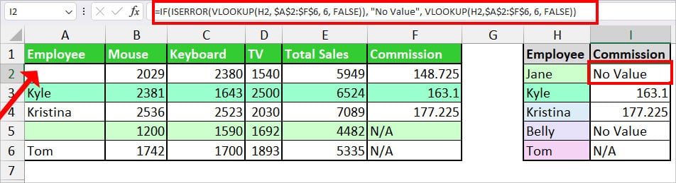
The formula returned No Value for our first cell. We then dragged the Flash-fill handle for the rest of the cells too.
Let us now see how the formula worked.
- VLOOKUP(H2, $A$2:$F$6, 6, FALSE): Firstly, the VLOOKUP searches lookup value “Jane” in Lookup table $A$2:$F$6 and returns Commission from the 6th Column. Since we specified the FALSE argument, the formula either returns the exact item or error. In this case, we got #N/A.
- ISERROR(VLOOKUP(H2, $A$2:$F$6, 6, FALSE)): Now, the ISERROR checks if the output returned by VLOOKUP has an error. Since there was #N/A, it returned TRUE.
- IF(ISERROR(VLOOKUP(H2, $A$2:$F$6, 6, FALSE)), “No Value”, VLOOKUP(H2,$A$2:$F$6, 6, FALSE)): Finally, the IF function, tests ISERROR(VLOOKUP(H2, $A$2:$F$6, 6, FALSE)) logical value which is TRUE. If the value is true, it results in “No Value.” Likewise, in case the Value is False, it returns the Commission Value. Hence, we got No Value.
Count the Number of Error Cells
Did you know you could count the number of cells that contains an error?
Well, you can do this with the ISERROR function and SUM functions nested together. It comes in handy when you need to report someone about the number of errors in a workbook.
Example: Let’s assume, you need to count error cells from I3:I4. To do so, we entered the formula as
=SUM(--ISERROR(I3:I4))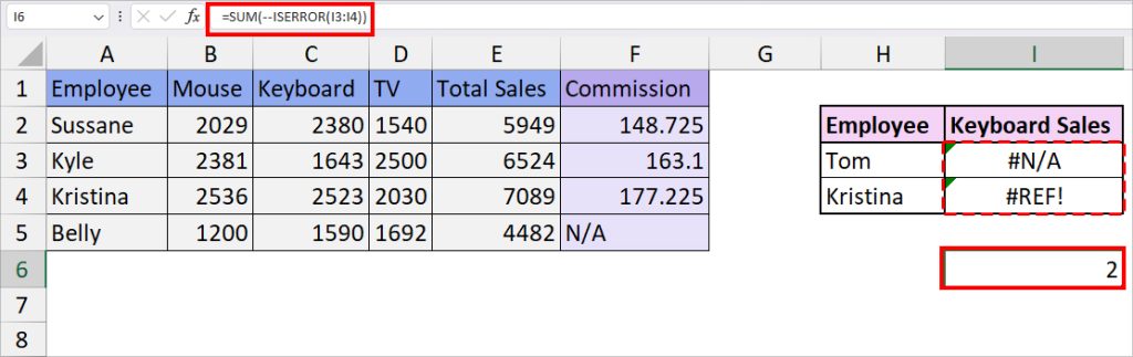
The formula returned 2.
Alternative to ISERROR Function
Above, we nested the IF function with the ISERROR function in one of the examples to return a value if there’s an error. But, instead of nesting them together, there’s an actual function named “IFERROR” to do this.
Excel’s IFERROR function returns a certain value when the cell/expression contains an error.
Syntax: IFERROR(value, value_if_error)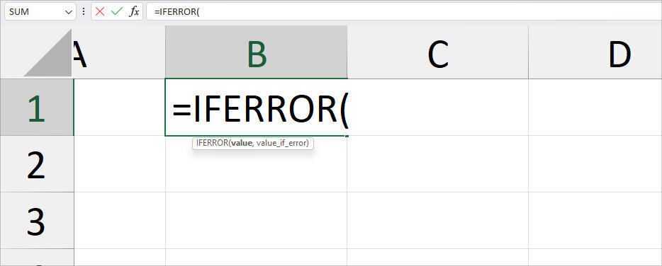
Similar Functions Like ISERROR
| Function | Syntax | Description |
| ISNA | =ISNA(value) | Tests and returns TRUE boolean if there are #N/A errors only. |
| IFNA | =IFNA(value, value_if_na) | Tests and returns a message when the value contains #N/A error. |