Excel’s INDIRECT function is one of the Lookup and reference functions. Its application ranges from creating an indirect cell referencing within sheets to different sheets. I personally use this function while inserting a dependent drop-down list in Excel. Unlike other functions, lookup functions can be a little complex to understand. So, here, you can find a beginner-friendly tutorial on the INDIRECT function.
What is an INDIRECT function?
An INDIRECT function returns the reference value of the text string you pass down in the formula. It indirectly references a cell via a messenger cell.
Now, you may have a query just like the other users. Why use the INDIRECT function when you can directly create a cell reference?
Well, the INDIRECT function locks the cell references you pass down in the formula. So, even if you insert or delete a new column/row, it’ll still return the exact value in the cell.
Also, this function is mostly used to dynamically reference a worksheet or a workbook. So, you can use this function whenever you wish to command the formula to refer to a different cell reference.
Arguments for INDIRECT Function
Before you check out the uses of the INDIRECT function, it’s important to learn the function arguments. You can pass down two arguments in the INDIRECT function which are ref_text and [a1]. Let’s see what each argument refers to.
Syntax: INDIRECT(ref_text, [a1])- Ref_text: A cell reference or named range.
- [a1]: Boolean to specify the reference style.
- TRUE: A1-style reference
- FALSE: R1C1 reference style
Remember, function arguments with [] parentheses are optional.
Although optional, as you need to specify a boolean of cell referencing style [a1] in the INDIRECT function, it’s better you know the difference between them. Most beginners might not be familiar with Excel’s cell referencing style.
The A1-cell Reference style is a default style in your Excel spreadsheet that you always get whenever you open a new workbook. Here, the style takes the Column Headers as letters like A, B, C, D, E, F, etc. Similarly, the ROW headers are formatted as numbers 1, 2, 3, 4, 5, etc. With A1 style, the cell reference name would be A2, B4, etc.
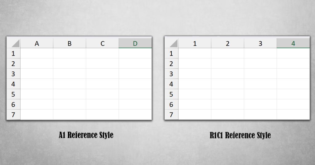
On the contrary, the R1C1 Reference style will take the Rows and Columns of your spreadsheet in numbers. Meaning, with this type of reference, the Column header such as A, B, C, D, E, etc will change into 1, 2, 3, and 4 just like the Row header. So, the cell reference name would be R1C1, R3C2, R5C3, etc. Here, R5C3 means the cell of the 5th Row and 3rd column.
Things You Should Know Before Using the INDIRECT Function
- An INDIRECT function is a “Volatile” Excel function. So, it could affect the worksheet’s performance during each recalculation.
- If you do not enter the cell reference style in the formula, the INDIRECT function takes “A1 style” as a default.
- As INDIRECT functions are Case-sensitive, it takes lowercase and uppercase words differently.
Examples of INDIRECT Function
To understand the INDIRECT function better, we have compiled a few examples below.
Example 1: Using a Cell Reference
Suppose, Cell A2 has a word named “Sheets.” On cell B2, we’ve entered “A2” as you can see in the given picture.
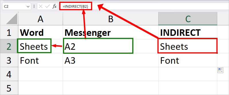
Now, if you enter =INDIRECT(B2) formula in cell C2, you’ll get Sheets as a result. Notice how the value in B2 was a messenger that indirectly referenced the value of A2 cells.
Example 2: Using Named Range
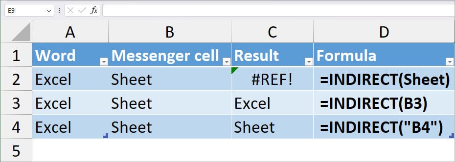
Let’s assume, we have “Excel” in Column A and “Sheet” in Column B. Let’s see the examples for using Named Range in the function from the given table.
| Example | Formula | Result | Description |
| 1 | =INDIRECT(Sheet) | #REF! Error | When we entered Sheet in the formula, it returned #REF! Error. This is because it does not have a reference to other cells. |
| 2 | =INDIRECT(B3) | Excel | This time the formula returned “Excel.” How? It’s because we named cell A3 as a Sheet. So, it is creating an indirect reference to Excel. |
| 3 | =INDIRECT(“B4”) | Sheet | In this case, we double-quoted the value of “B4” in the formula. So, the INDIRECT function is actually looking for the value inside the cell instead of a reference. As a result, the formula returned Sheets and not Excel. |
Named cell ranges are also easier to use when you are nesting the INDIRECT function with other functions. Let’s take a look at another example.
Example: COUNTA and INDIRECT
In the given example, we have a list of countries’ names from cells B1 through B5. We named these cell ranges (B1:B5) as Countries from the Name box. Suppose, we want to count the cell ranges. To do so, the formula would be
=COUNTA(INDIRECT(D1))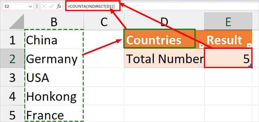
In the above formula, the messenger cell is D1 “Countries.” So, the INDIRECT function first returns the value from cell B1 through B5 cell ranges. Then, the COUNTA function counts the total number of cells and returns 5.
Example 3: Concatenate Cell Reference and Text
When using the INDIRECT function, you can also pass down the two cell references concated together. For example, to reference the value of cell C4, you can enter the formula as
=INDIRECT("C"&4)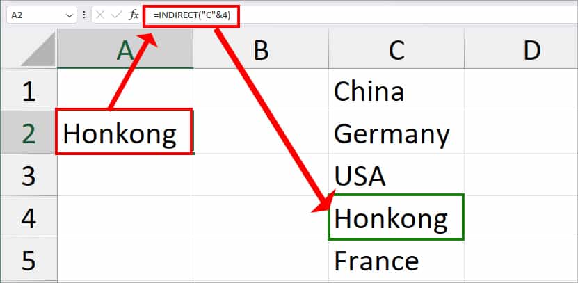
The formula basically concates Column C and Row 4 with the ampersand operator in between. Then, it returns the value of C4 which is Hongkong.
Applications of INDIRECT Function
Create a Reference to Another Sheet
INDIRECT functions have much more dynamic applications than just creating cell references within the sheet. For Instance, you could create a dynamic reference to another sheet, also called a 3-D referencing in Excel.
Normally, you’d use the =(Your Sheet name)!(Cell ranges) formula to link cells of a different worksheet. But, if your Sheet name has two or more words, it adds up a space in between the name. Instead of =Sheet4!B2, your formula will look something like this =‘Countries Name’!C2.
But, if you enter a Sheet name and address in cells, all you have to do is concatenate together. Note that you must use double and single quotation marks and exclamation marks for the cell with the Sheet name to format it as a sheet.
Example: Here, we’ve entered the Sheet name, Column name, and Row number of a different sheet in cells A2, B2, and C2. We will use and concate these cells using the ampersand symbol in a formula to create a worksheet reference. For this, we entered the formula mentioned in the box which returned France as a result.
=INDIRECT("'"&A2& "'!" &B2&C2)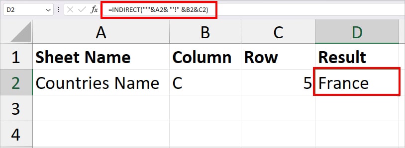
Reference Drop-down list
In Excel, you can also use the INDIRECT function to create a dependent drop-down list. Let’s take an example we have two laptops and their model in Columns C and D. Before you use INDIRECT to reference the drop-down list, there are two preliminary steps you need to perform.
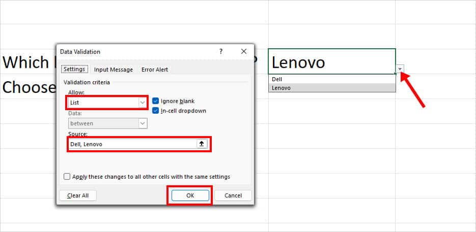
- Create a first Drop-down list. From Data tab, click on Data Validation. On the Settings tab, pick List for Allow. Then, type in Dell, Lenovo in the source. Once you click OK, you’ll have the drop-down list.
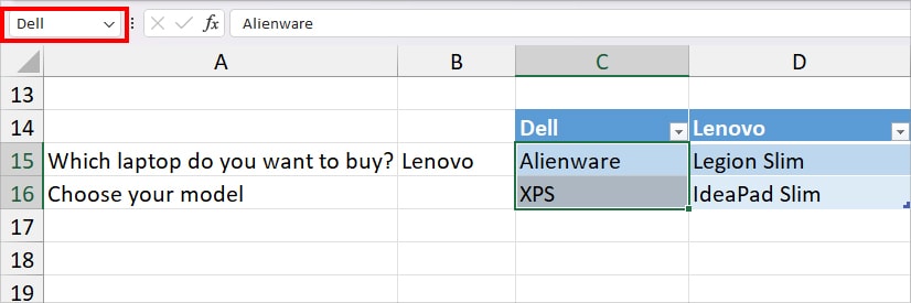
- Name the cell ranges containing the model with the exact name as the first drop-down list. For Instance, I selected cell C15:C16 and typed in Dell in the name box. Similarly, named cells D15:D16 as Lenovo.
Now, since we have the required criteria to reference cells, we will use the INDIRECT function now.
- Select a Cell to add a dependent drop-down list.
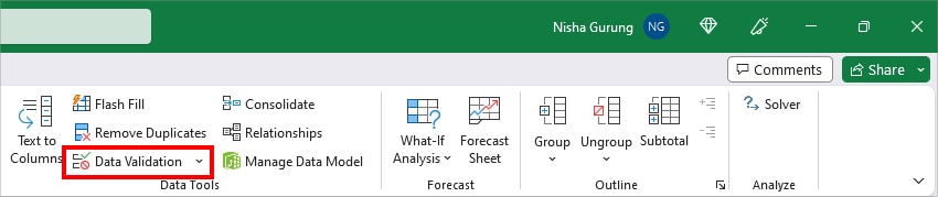
- From Data tab, select Data Validation in Data Tools group.
- On Data Validation window, stay on the Settings Tab. Below Allow menu, pick List and enter
=INDIRECT($B$15)formula in Source.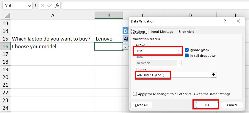
- Hit OK.
- Now, if you select Lenovo laptop in the first drop-down, you’ll only have Legion Slim and IdeaPad Slim to choose from in the second drop-down.
Avoid #REF! Error When Using INDIRECT Function
There are a number of reasons you may encounter #REF! Error when using the INDIRECT function in Excel. You’ll get this error when the ref_text argument is an invalid cell reference, missed double quoting in ref_text, or entered cell range beyond the Row Limit. To avoid this error, check and ensure you pass down the correct cell reference in the formula.