Whenever you use the VLOOKUP function, it either returns an exact/partial match value from the lookup table or a cell error if the value isn’t found.
But, if you use the IFERROR and VLOOKUP nested together, you can manipulate the formula to ignore the error and return any value you want.
For example, instead of a #N/A, you can have “No Data” text, a blank cell, or a different output in the formula cell. I’d definitely say it is also one of the tricks to keep your Excel sheet clean.
So, let us learn how to best use IFERROR in VLOOKUP with examples.
Before we dive into the applications, let’s quickly recap the function syntax for both IFERROR and VLOOKUP.
| Function | Syntax | Description |
| IFERROR | =IFERROR(value, value_if_error) | It substitutes the result with a specified value when the formula returns errors like #NAME?, #N/A, #NULL!, #REF!, etc. |
| VLOOKUP | =VLOOKUP(lookup_value, table_array, col_index_num, [range_lookup]) | Returns an item for the lookup value from the specified column of lookup range. |
Substitute Error with Value
Firstly, you could use the IFERROR in the VLOOKUP function to substitute the error with the Value you want.
When your VLOOKUP function is not working, you might encounter several cell errors. But, since the #N/A error is the most popular one, we will use it as an example.
Example:
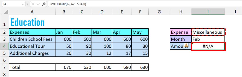
Suppose, I want to return the Miscellaneous amount for the month of February. If I enter =VLOOKUP(I2, A2:F5, 3, 0), I’ll get #N/A error. This is because there is no Miscellaneous expense category in the specified lookup table.
But, if I use the IFERROR and VLOOKUP together, I can return “No Expense” as an output. To do so, I’ll use the given formula.
=IFERROR(VLOOKUP(I2,A2:F5,3,0),"No Expense")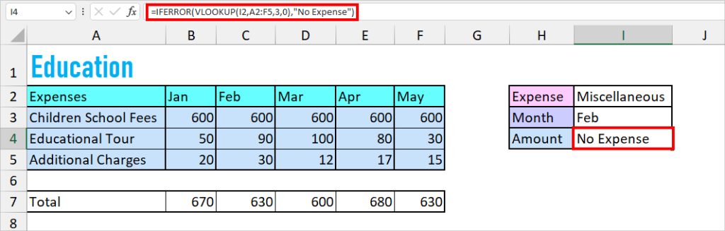
In the IFERROR formula above, VLOOKUP(I2, A2:F5,3,0) is the value, and “No Expense” is the value to return when there’s an error.
Remember, the correct way to reference Text strings is to always enclose them within the double quotation mark. If you don’t, you’ll face the #NAME? error.
Return Blank Cell With VLOOKUP
If you do not want to return any values and rather wish to keep the error cell blank, it is also possible with IFERROR and VLOOKUP.
Example:
Let us again take the same example as above where VLOOKUP returns #N/A as there is no Miscellaneous expense. This time we will substitute the #N/A with the null string. To do that, my formula would be
=IFERROR(VLOOKUP(I2,A2:F5,3,0),"")Return Value From Different Lookup Table
One of the drawbacks of the VLOOKUP function is it can take only one lookup value and table array at once. But, with the nested formula of IFERROR and VLOOKUP, you can overcome this limitation. It’s kind of similar to using VLOOKUP with multiple criteria.
Example:
Suppose, I have two lookup tables of Household Expenses for the month of January, February, March, April, and May. Take, for instance, I want to randomly look for the Grocery expense amount for the month of May which could be in any of the lookup tables.
For that, I’ll use this formula.
=IFERROR(VLOOKUP(J3, A3:H7, 6,0), VLOOKUP(J3, A11:H17, 6, 0))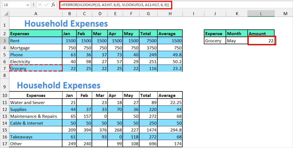
Here, the formula is pretty simple. If the first value VLOOKUP(J3, A3:H7, 6,0) results in an error, the IFERROR will return the value of VLOOKUP(J3, A11:H17, 6, 0). As a result, we got 22.
Keep in mind, in case there was no Grocery expense, it would eventually result in a #N/A error. So, to avoid errors, you must have an exact or approximate value in either of the lookup tables.
Return Different Output
There can be instances when you might want to return the result for a second lookup value from the same table array when the first item is not found. You won’t be able to achieve this just by using the VLOOKUP function.
So, we will now learn how to return a different output through the given example.
Example:
Let us assume that I have a lookup table with the teacher’s number. Using the IFERROR and VLOOKUP, I want to return the number for Principal if there is no value for Tuition Teacher. For this, I used this formula:
=IFERROR(VLOOKUP(E3, B3:C6, 2, 0), VLOOKUP("Principal", B3:C6, 2, 0))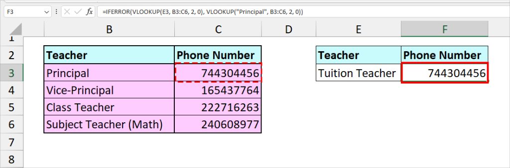
This formula uses the same logic as we mentioned for different lookup tables above. However, this time our lookup table is the same.
Instead, we have specified VLOOKUP to return an output for another lookup value which is “Principal” whenever there’s an error.
Alternatives to IFERROR With VLOOKUP
You can also achieve the same goal as IFERROR with VLOOKUP using the given alternatives. Check out the syntax and try using them as per your situation.
| Function | Syntax | Why this alternative? |
| IF, ISERROR, and VLOOKUP | =IF(ISERROR( VLOOKUP(lookup_value, table_array, col_index_num, [range_lookup])), “value_to_return_if_error”, VLOOKUP(lookup_value, table_array, col_index_num, [range_lookup])) | Use this if you have a dedicated “value to return when there is a VLOOKUP error” and an “item when there is no VLOOKUP error.” |
| IFNA and VLOOKUP | =IFNA(VLOOKUP(lookup_value, table_array, col_index_num), value_if_na) | Use this when your VLOOKUP formula returns only the #N/A error. |
| XLOOKUP | =XLOOKUP(lookup_value, lookup_array, return_array, [if_not_found], [match_mode], [search_mode]) | A major advantage is you do not have to nest formula. |