Although Excel’s XLOOKUP function is powerful enough to return sequential rows from the lookup table, it does not return multiple matches for a single lookup value.
Meaning, you would get only the first match based on the argument you pass on like the Exact Match, Approximate Match, Partial Match, Search Modes, and so on.
But, to overcome this limitation and return all matches, we have several workarounds like the FILTER function, TEXTJOIN and IF function, etc.
Using FILTER Function
The FILTER Function returns an array from the Lookup table depending on the True or False boolean. So, we will use this function to look for all the matches of a single lookup value and return the output.
Generally, the syntax for the FILTER function is:
=FILTER(array, include, [if_empty])But, to return all matches, this is the formula we will use.
=FILTER (return array, lookup array = lookup value)Example:
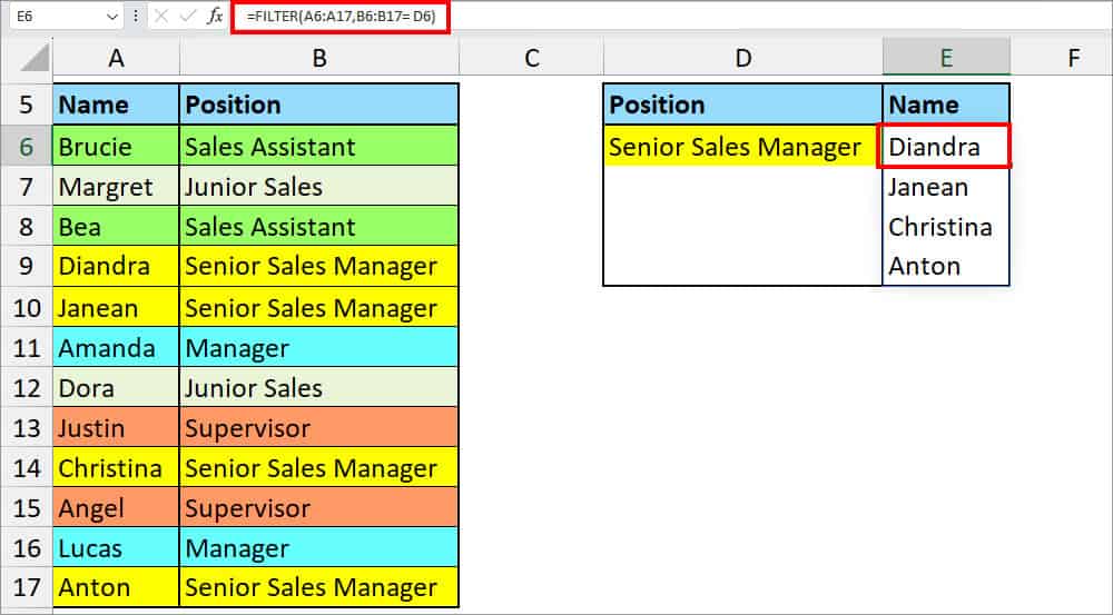
Here, I have Employee Names and their Positions. Suppose, I want to return all Names with the “Senior Sales Manager” Title.
For that, I will enter this FILTER formula.
=FILTER(A6:A17, B6:B17= D6)
As a result, I got Diandra, Janean, Chrsitna, and Anton. The formula looked for lookup value in cell range B6:B17. Then, returned the names from range A6 through A17.
If your FILTER function is not working, we have a detailed guide on how to fix it.
Using TEXTJOIN and IF Function
In the above example, we returned all values with the exact match in an array. But, instead of spilling the results in an array, you can also return the output in the same cell separated by a comma.
To accomplish that, we will opt for the TEXTJOIN and IF functions nested together.
Formula:
=TEXTJOIN(“delimiter”, TRUE, IF(lookup value = lookup array, return array, value if false))Example:
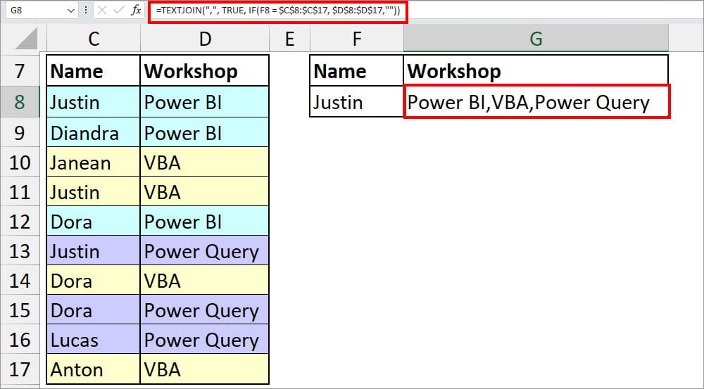
Suppose, I have lists of Names and the Workshop these people are attending. From that data, I want to find out what workshop “Justin” will take part in.
To know, I used the TEXTJOIN and IF formula given in the box below.
=TEXTJOIN(",", TRUE, IF(F8 = $C$8:$C$17, $D$8:$D$17,""))
In the formula cell, I got Power BI, VBA, Power Query for Justin.
So, how did the formula work? Let’s check it out below.
- IF(F8 = $C$8:$C$17, $D$8:$D$17,””): Here, the IF function will return the value from $D$8:$D$17 if the F8 = $C$8:$C$17 condition is TRUE. Similarly, it would return, “” when the logical test is FALSE.
- TEXTJOIN(“,”, TRUE, IF(F8 = $C$8:$C$17, $D$8:$D$17,””)): Now, the TEXTJOIN combines all the text strings returned by the IF formula which is separated by a comma delimiter.