When working with data in Excel, you should be familiar with the basic arithmetic operators like: (+, -, *, /). Although it looks intimidating, Excel has made this so simple that even the most inexperienced users can catch up in a matter of minutes.
Here, we will discuss one of these operators : Subtract. Unlike multiplying in excel, there aren’t many ways you could subtract values.
The minus or hyphen (-) operator can be used in the same way as you would in paper. With this, you can find the differences between values, columns, dates, times, etc.
There is no specific function for subtraction, as there is for SUM or PRODUCT. But we have a workaround which we will discuss later in the article.
Subtract Numbers
Suppose, you want to subtract any two numbers, the formula would be
=number 1 - number 2
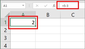
Example: To find out the difference between 5 and 3, enter =5 - 3 in a cell. You will get 2 as result.
Subtract Relative Cell Reference
Instead of typing values one by one, try referring to a cell. This way, you could write the formula once and double click at the edge of the cell and the formula gets copied to the entire row with it’s calculated value.
The following formula works if you have a Relative cell reference. Meaning, both the referring cells will move once the value is copied down.
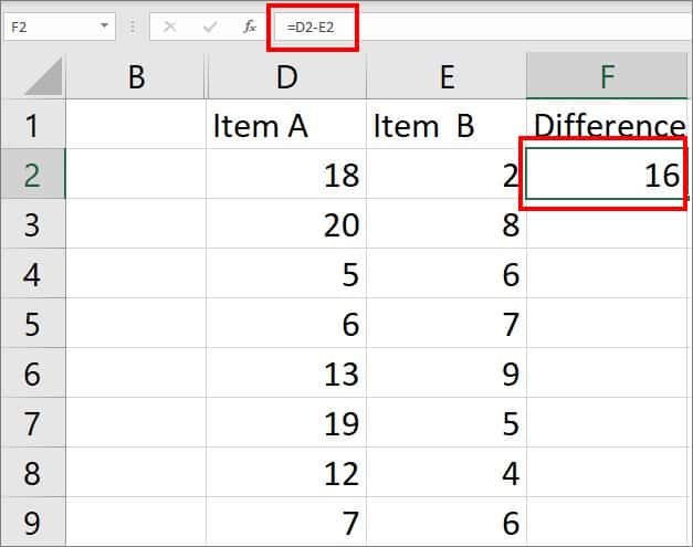
Example: For subtracting Item A and Item B, we will enter =D2 – E2 in the F2 cell. It subtracts 18 – 2. So, you get 16 as a result.
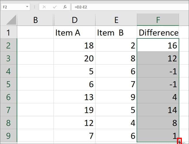
Now, when you hover the cursor over the bottom of cell F2, a small plus sign should appear. Drag down the Plus Sign to fill the ranges with the same formula.
Note: In case you get the date format in results, change it to General from the Number section of the Home Tab.Subtract Absolute Cell Reference
Let’s assume you need to get the difference between the numbers of columns and a constant number.
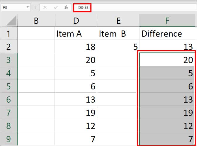
To subtract the whole Column D with the number 5 of the E2 cell, we will use the =D2 - $E$2 formula. In the formula, we have added dollar signs in the E2 cell to change it to an Absolute cell reference. By doing so, all the cells of column D will refer to only cell E2 for subtraction.
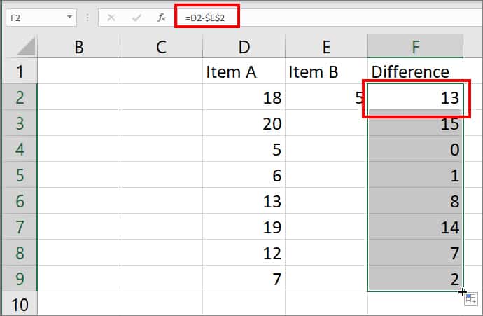
If you do not lock it, the cell reference will change respectively when you flash-fill the formula. For Instance, D3 will subtract cell E3. As cell E3 is empty, you’d get the Exact number as an outcome.
Using SUM Function
Although Excel lacks a dedicated function for subtracting values, there is a workaround. Simply convert one of the values to a negative number and add the two values together using the SUM function.
Syntax: =SUM(A1,-B2)
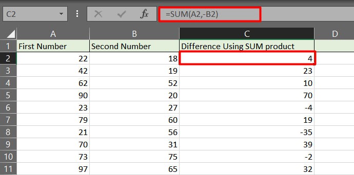
If your data has a negative number, the above formula may not be effective. This is because when two negative signs combine, it will add numbers and you may get a different outcome. To avoid such case, you could use the absolute function.
Syntax: SUM(A1,-ABS(A2))
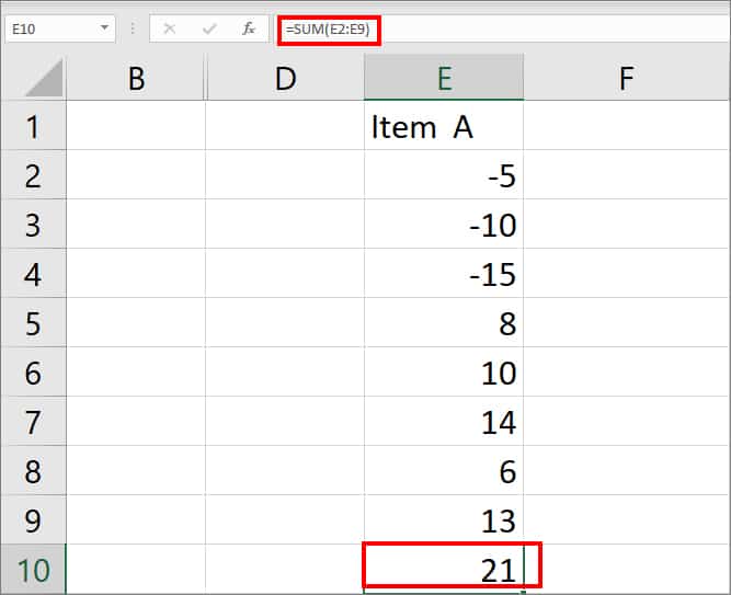
Or, you could take advantage of the situation and add all negative numbers. This will provide you with the exact difference.
Syntax: SUM(number1,[number 2]...)
Let’s see how we used this function in the given example. According to our data, the formula would be=SUM(E2:E9) . Firstly, enter =SUM in E10 cell. Insert open parenthesis and select cells from E2 to E9. Then, close the parenthesis and press enter.
Subtract Percentage
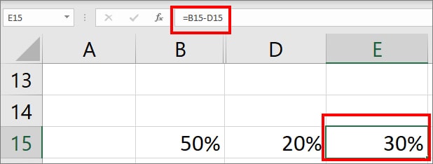
For subtracting percentages, you can use the same formula that has cell references. For Instance, to get the difference between 50% and 20%, enter =B15-D15 formula in E15 as per the given data.
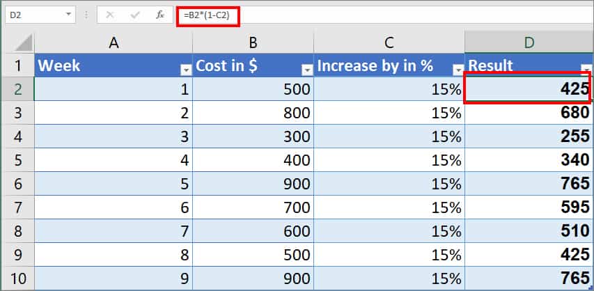
But, if you have to decrease a given number by a percentage, there’s a different formula for it i.e. =Value * (1 - %).
Suppose, you want to reduce Column B by Column C percentage. To calculate this, enter the =B2*(1-C2) formula in the D2 cell. As per the PEMDAS rule, Excel will first calculate the value inside parentheses i.e. (1-0.15 = 0.85). Then, it will multiply the outcome by the number (0.85 * 500 = 425).
Subtract Date
You can also subtract dates to find out the duration between the two given dates. For this, use the given formula,
=End_Date - Start_Date
According to the data, enter =C15-B15 on Cell D15. The result will show the number of days. Here, C15 is the end date and B15 is the start date.

Subtract Time
For users who want to calculate the total time spent, you can use =End_Time-Start_Time formula.
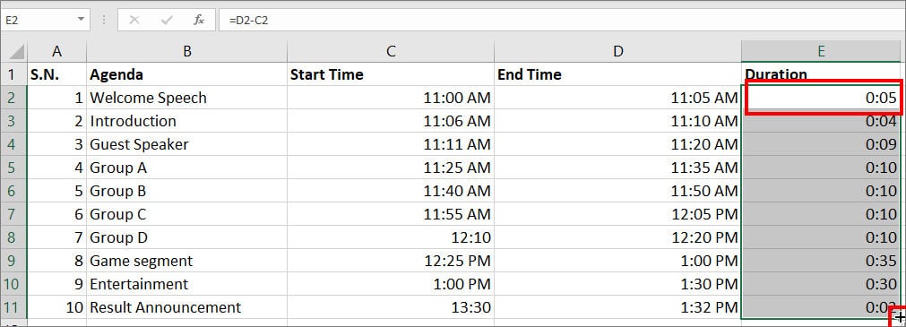
- On Cell E2, enter
=D2-C2. (D2 is end time and C2 is start time)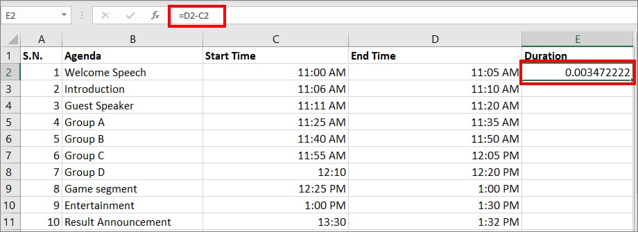
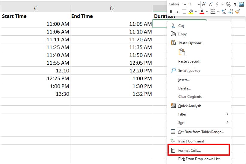
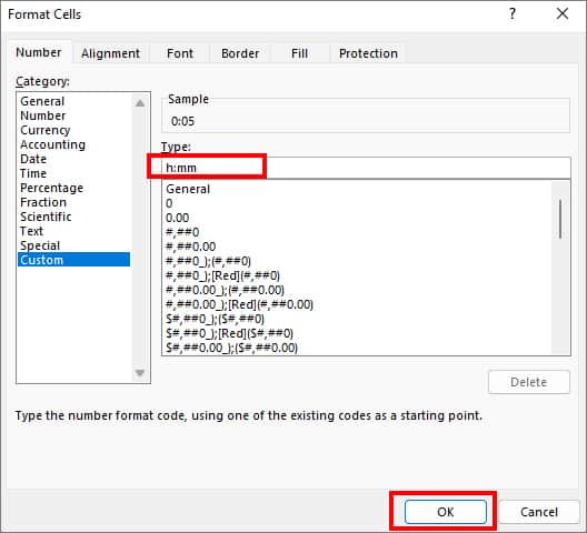
- Now, right-click on E2 cell and choose Format Cells.
- From the Number Tab, go to Custom Category.
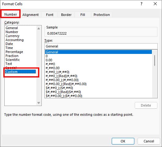
- Under Type, enter h:mm and click OK.
- Drag the Fill handle to apply the format to other ranges too.
If you have to subtract time exceeding 24 hours, on Cell E33, type in =(D33-C33)*24. You should get the number of hours.
