Your Excel cell’s default height and width is 15 and 8.38 points respectively. When the data exceeds the cell’s default width, it either spills to the next cell or stays hidden depending on if you have data in the adjacent cell.
While you can autofit the cell to resolve this issue, your spreadsheet may look odd if the remaining cell values in the column aren’t the same width. Besides, if you’ve entered a sentence, autofitting the cell will widely stretch your column.
Instead, you can insert line breaks within your cell to start a new line within the Excel cell. In this article, we have covered how to insert these line breaks while entering and after entering data.
Start a New Line While Entering the Data
If you haven’t started entering your data, you can use the line break shortcut to start a new line in your cell. The shortcut to enter this line break depends on if you’re using Excel on Windows or Mac.
Start entering your data. When it’s time to move to the next line, use the following key combination:
WINDOWS
ALT + ENTER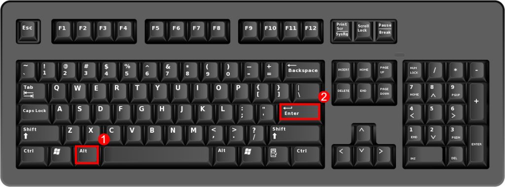
MAC
CONROL + OPTION + RETURN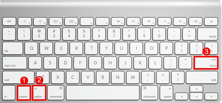
Start a New Line After Entering the Data
If you have already entered your data and are now looking to add line breaks in existing data, you can use Excel’s wrap and Find and Replace tools.
Additionally, if you’re into creating formulas, we have a formula using the TEXTJOIN and CHAR to insert a line break.
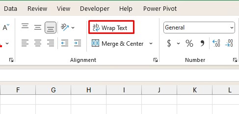
Wrap Text Tool
The wrap text tool in Excel is my go-to when it comes to adjusting data within the cell. Excel will automatically change the height of your cell to adjust your cell content when you use the tool.
- Select the range with your data.
- Head to the Home tab.
- In the Alignment section of the ribbon, select Wrap Text.
Find and Replace
You can use the Find and Replace tool if you want to substitute a specific character with a line break. For example, you can use this tool to locate the comma symbol (,) and replace it with a line break within your data.
- On your keyboard, use Ctrl + H.
- In the Find what section, enter the symbol you wish to replace with the line break. In our case, this is the comma sign (,).
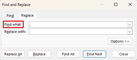
- Next to Replace with, use the Ctrl + J key combination. Make sure there is a blinking dot after you use the combination.
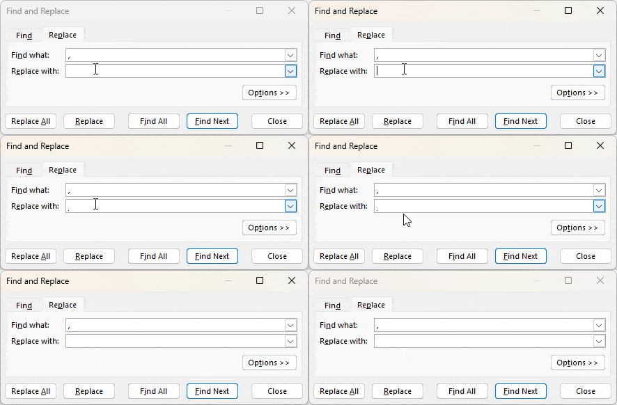
- Select Replace all.
Nest CHAR Inside TEXTJOIN
You can use the TEXTJOIN and CHAR functions to create a formula to insert line breaks.
This is the syntax you must follow when using the TEXTJOIN function in a formula:
=TEXTJOIN(delimiter, ignore_empty,text1…)| Argument | Data Type | Description |
| delimiter | CHAR | The separator in between the merged texts. |
| ignore_empty | BOOLEAN | Enter TRUE (1) to ignore empty cells and FALSE (0) to include empty cells. |
| text1 | TEXT | The first text or reference you wish to merge. To enter the remaining texts, use the comma symbol and start referencing. |
Here’s how you can enter the CHAR function when constructing a formula:
=CHAR(number)You can enter a special character using the CHAR function by referencing its ASCII code in the number section. In our case, the ASCII code for line break is 10. Therefore, we will be passing 10 as our reference inside the CHAR function.
Here’s how we created a formula using TEXTJOIN and CHAR to merge three cells in columns A, B, and C with line breaks.
=TEXTJOIN(CHAR(10),TRUE,A2,B2,C2)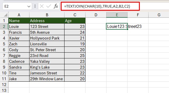
Once I entered my formula, I used Flash Fill to apply the formula to the remaining cells in column D. Then, go to the Home tab and select Wrap text to insert the line breaks.
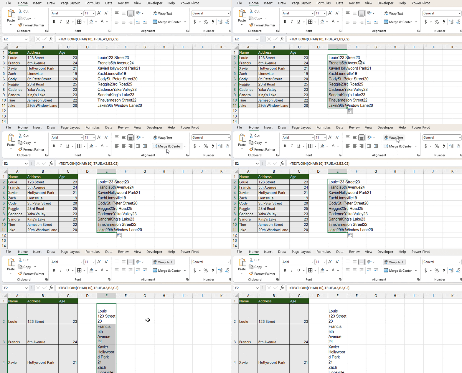
The Wrap Text tool will break lines only from the area where you’ve entered CHAR(10) as the delimiter.