If you have color-coded cells in Excel, you may wish to organize the data based on those colors.
For Instance, keep all the Green cells with “Completed” status at the top. Or, a cell filled with Yellow with “Average Numbers” in the middle.
In addition to making your sheet aesthetically appealing, sorting cells by color will also help you in creating data visualization like a heat map.
What I like most about Excel’s Sort feature is that it allows you to make a custom Color order.
Now, let’s find out how you can sort cells by color in Excel.
From Context Menu
If you just need to sort your data based on one color, do it from the Context Menu. It’s easier as you can also see the items in that cell.
Simply, right-click on the Cell with color. Head to Sort. Then, choose any one given option.
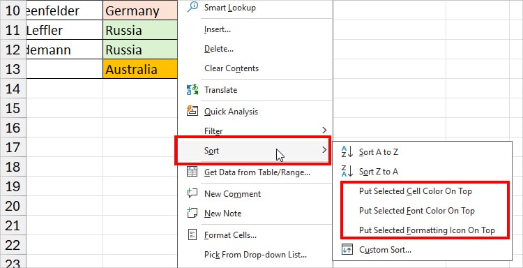
- Put Selected Color On Top: Organize values based on filled cells.
- Put Selected Font Color On Top: Reorder values based on the Font Color.
- Put Selected Formatting Icon On Top: Rearrange the column based on the Conditional Formatting Icon.
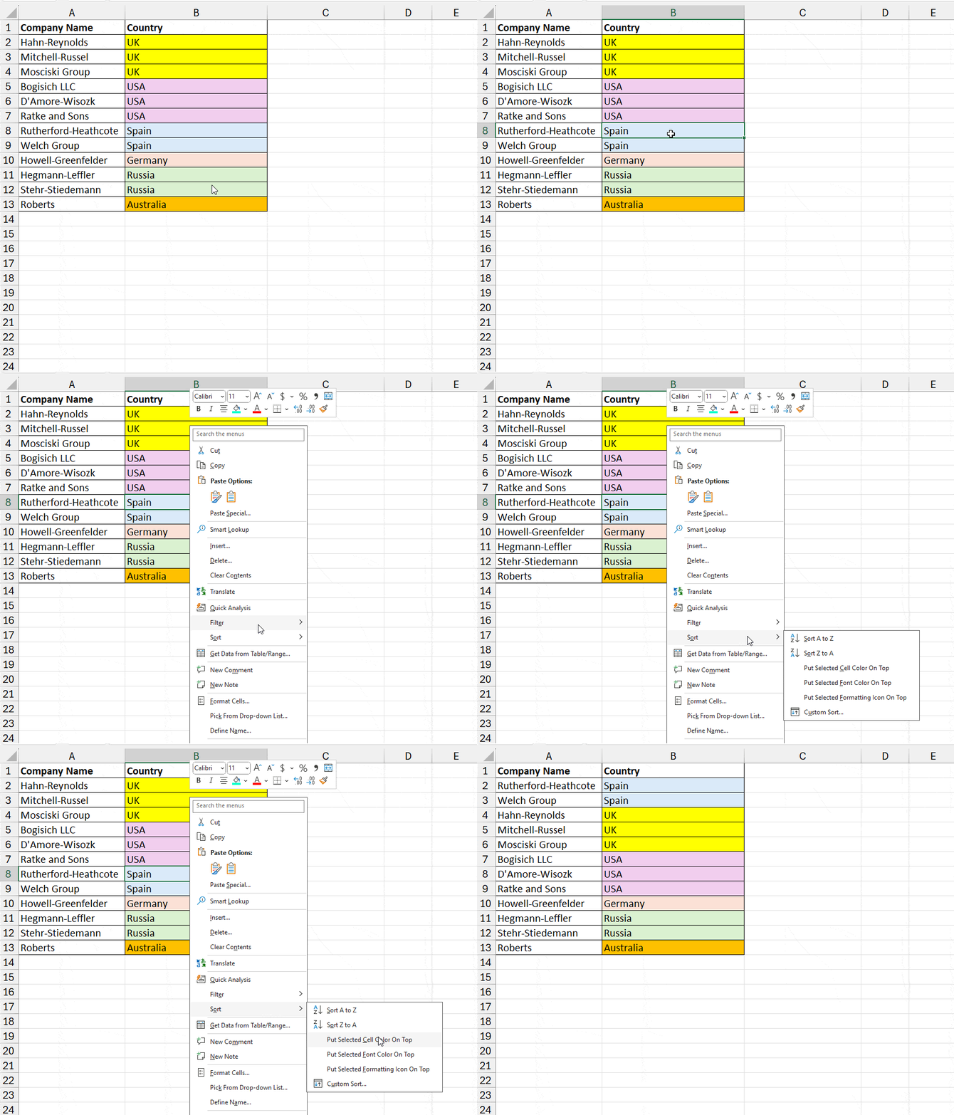
Suppose, if I chose Put Select Color On Top, Excel keeps the blue color at first. Similarly, the Yellow color that was at the beginning will move down.
Using Filter
From my experience, using a context menu is only simpler when you have smaller data. For a huge dataset, it can be a hassle to locate the specific shaded cell in thousands of columns.
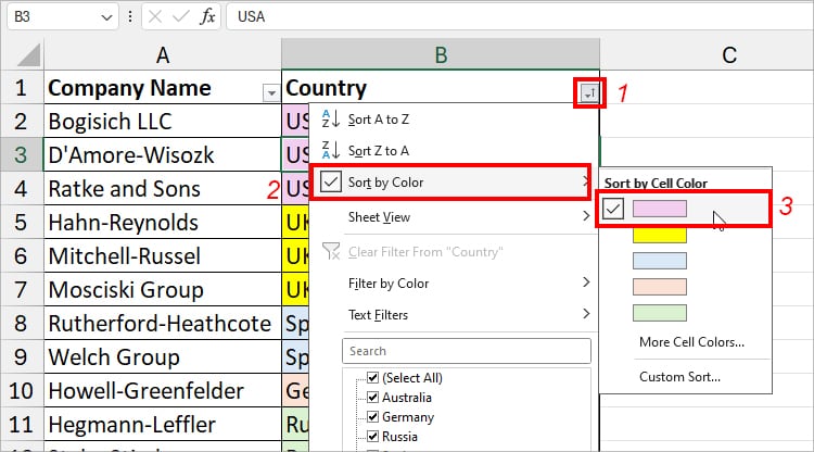
During such a case, I prefer the Sort by Color option in the Filter tool. It is another quickest way to reorder the column by the cell or font color.
Firstly, enter these shortcut keys to turn on the Filter.
Shortcut: Ctrl + Shift + LNow, click on the Filter button. Hover your cursor over Sort by Color and choose a Color. Remember, the one you pick will be at the top.
Using Sort Menu
In the both above methods, we can put only the chosen shade at the beginning. But, if you have multiple colors and need to define your color order, the SORT menu is the best.
For Instance, you could put Green at first, Yellow on second, Red on third, and so on.
The best part is you could also rearrange the rows based on the color.
Sort By Cell Color
Example1: Sort Column
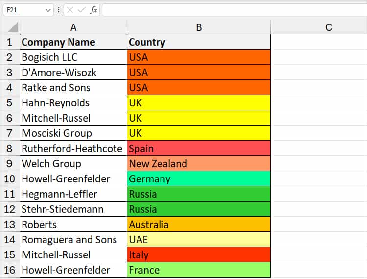
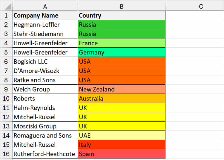
Suppose I have lists of Company Name and Country. The Countries are highlighted with 10 different colors. Here, I will set my own color order to sort by.
- Select the Data Range.
- From the Data Tab, click on Sort Button.

- On the Sort dialogue, choose Column Header in the Sort by.
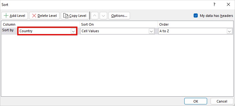
- On Sort On, pick Cell Color.
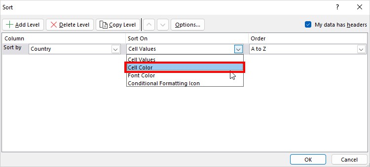
- Select the Color and choose Order. Here, I picked On Top.
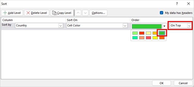
- If you have multiple Colors, hit on Add Level. Set the Then by, Sort On, and Order. Once you’re done, hit OK.
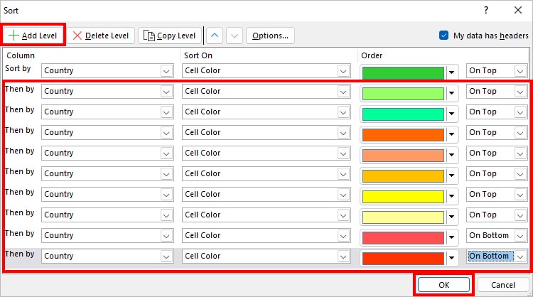
- You’ll have sorted colors as specified.
Example 2: Sort Row
- Select your data.
- Head to the Data tab and click on the Sort.

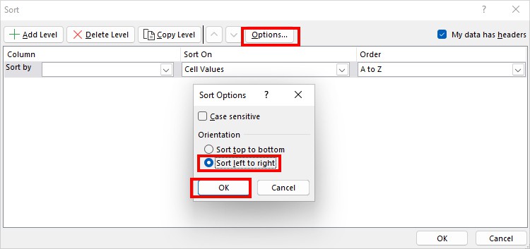
- Click Options. On the Sort Options dialogue, select Sort left to right. Click OK.
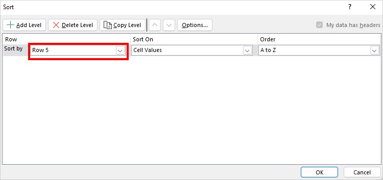
- Expand the drop-down for Sort by and pick Row.
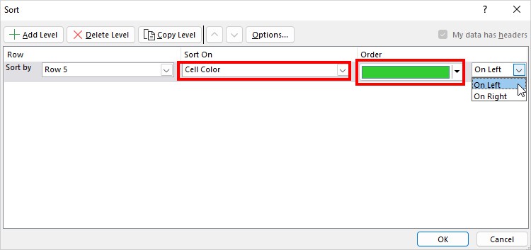
- For Sort On, choose Cell Color. On Order, pick Color and select On Left or On Right.
- Just like above, click Add Level. Set your Then by, Sort On, Order, etc.
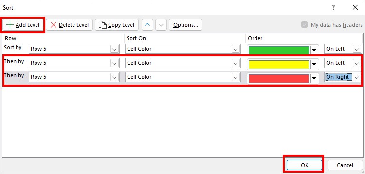
- Finally, hit OK. Excel Sorts rows as specified.

Sort By Font Color
Sometimes, instead of the Cell color, you may have a different font color to separate the values. To rearrange the items by the Font Color, here’s how to do it.
As an example, I have mentioned how to sort for columns. If you have highlighted a row, take a reference from Example 2 above. Make sure you change the Sort On to Font Color.
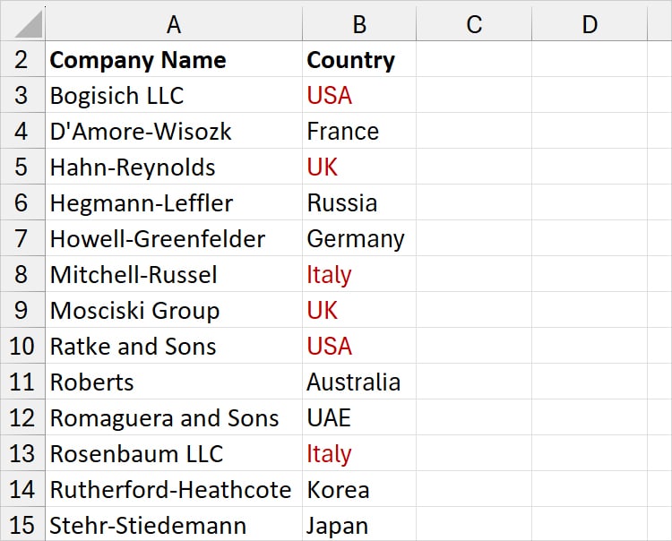
- Firstly, select your data.
- Press
Alt + A + SSRibbon Shortcut to open Sort. - On Sort by, choose a Column Header.
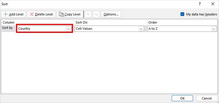
- Pick the Font Color option in the Sort On menu. Select the Color and choose the Order.
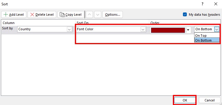
- Click OK.
Sort By Conditional Formatting Icon
Next, you can also sort the cells based on the Conditional Formatting icons. It could be any icon like directional, shapes, indicators, ratings, etc.

- Select Cell ranges.
- From the Data tab, click on the Sort button.
- On Sort by, pick Column Title.
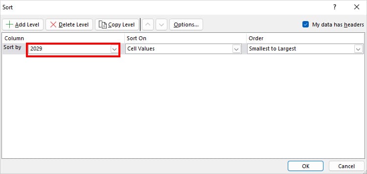
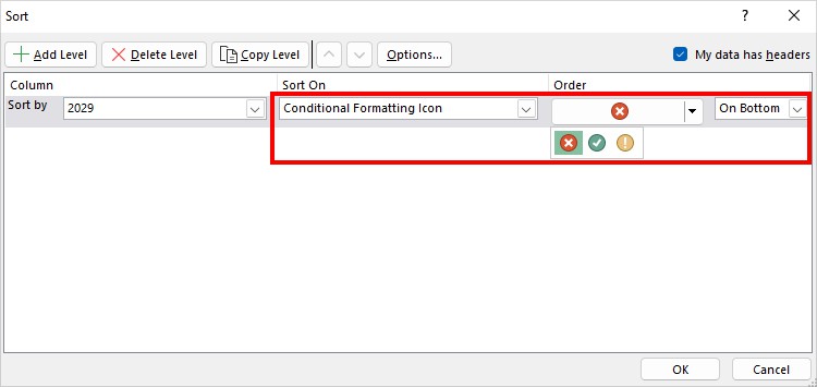
- Then, select the Conditional Formatting Icon in Sort On. Pick the Icon and choose your Position.
- Once you’ve added other levels, click OK.
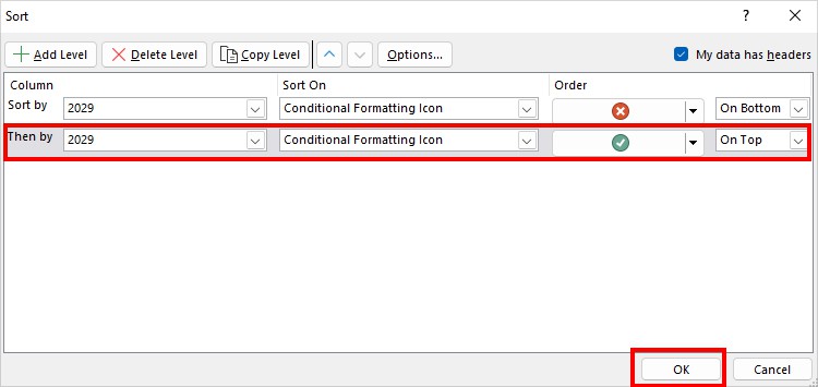
- Here’s the sorted data.
