How to Remove Parentheses in Excel

Round brackets, commonly known as parentheses in Excel, are used primarily in a formula or included in a cell value to add more information.

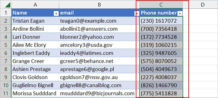
While often useful, the parentheses along with any text/number are sometimes optional or even unnecessary. Thus, you are better off without them in cases, like a phone number, (821) 2762360.

Depending on your specific case, different built-in functions and tools like the Find and Replace and SUBSTITUTE functions can help you remove them completely or replace them with another character like a dash, comma, or similar. Let’s learn more about them in the article.

Using Find and Replace

As the name suggests, the Find and Replace tool selects and replaces certain characters (numbers/texts) with another preferred one.

Additionally, there’s a special wildcard character, * , which helps to find and select any number of characters. 

1. Select the cell range that contains the values with parentheses. To select all cells at once, use the shortcut key Ctrl + A.
   
2. Press Ctrl +H.
3. On the Find and Replace prompt, type ( next to the Find what field.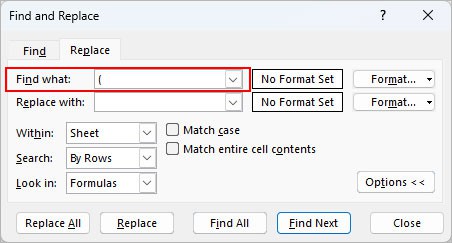
   
4. Click Find Next to individually go through each cell that will be selected.
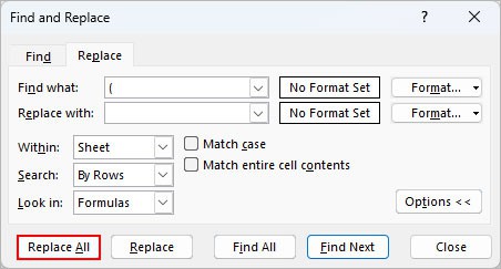
5. To replace the parenthesis with another character like a dash, type it in the Replace with field. Otherwise, leave it empty.
6. Click Replace All to remove every parenthesis character, ( .
   
7. Now, to remove the other parenthesis character, ), repeat the above steps. While doing so, make sure you enter ) in the Find what field.

Using Flash Fill

The Flash fill is a basic, yet powerful tool, that can save tons of time for various tasks like removing parentheses, without using any kind of formula.

It works best when the values inside a column follow a similar pattern. So, it likely won’t work as expected if you use it on values with different patterns, like 351(646)135-6452 and (319) 1060215, as their parentheses lie in different positions.

1. Create a helper column to store values without parentheses.
   
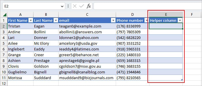
2. Select the first cell of the new column. Then, manually type the value without the parentheses such as 176 8336999 in the above image.
3. Press Enter and start typing the next value.
4. Once Excel suggests and fills other cells based on the pattern, press Enter.
   

Using SUBSTITUTE Function

The SUBSTITUTE function, well, substitutes a character with the new character you specify in the formula. It works like the Find and Replace and can be treated as a formula version of the tool.

Syntax:
=SUBSTITUTE(text, old_text, new_text)

Where,

• text: cell reference containing the specific text or character
• old_text: text or character that’s supposed to be substituted
• new_text: text: text or character that will replace the old_text

1. Add a  helper column to store values without parentheses.
2. Type the following formula in the first cell of the new column and press Enter. The mentioned formula first replaces the opening parenthesis with an empty string. Then, it replaces the closing parenthesis in the D2 cell.
   =SUBSTITUTE(SUBSTITUTE(D2,"(",""),")","")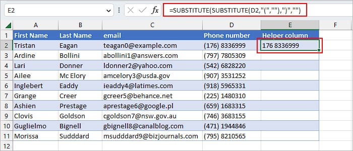
   
3. Drag the fill handle down the column to fill other cells with similar output.
   

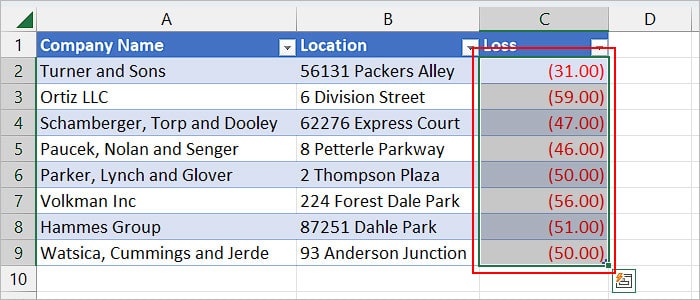
Using Custom Number Formatting

If you have set a number formatting that uses brackets to denote negative numbers, then a value like -10 is displayed as (10) in Excel.

To remove parentheses for such numbers, you simply set a different number formatting as follows.

1. Select the cell range containing negative numbers.
   
2. Press Ctrl + 1.
3. On the next prompt, select the Number tab.
4. Then, select Number under the Category section.
5. On the right pane, choose the format that doesn’t include parentheses such as -1234 or similar.
   
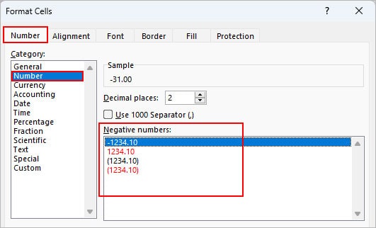
6. Click OK.

Using VBA

Another way to remove parentheses from your worksheet is to use a VBA code. Once you insert it into the worksheet and run it, Excel automatically removes all the existing parentheses from the selected cells.

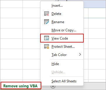
1. Select the cell range containing parentheses. To select all cells at once, press Ctrl + A.
2. Right-click on the active worksheet and select the View Code option.
   
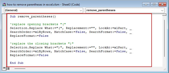
3. On the next window, copy and paste the following code.
   
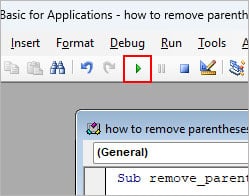
4. Then, press F5 or click the Run button below the top menu bar.

Sub remove_parentheses()

'replace opening brackets "("
Selection.Replace What:="(", Replacement:="", LookAt:=xlPart, _
SearchOrder:=xlByRows, MatchCase:=False, SearchFormat:=False, _
ReplaceFormat:=False

'replace the closing brackets ")"
Selection.Replace What:=")", Replacement:="", LookAt:=xlPart, _
SearchOrder:=xlByRows, MatchCase:=False, SearchFormat:=False, _
ReplaceFormat:=False

End Sub