While importing data in an Excel sheet, you might receive the numbers and text strings together in the same column. For Example, it could be the combined record of Student’s names and IDs like Ivan (5374). Or, just the numbers jumbled up in the texts like 1A5B3C2D.
Nonetheless, if the numbers do not add any value to texts, it is best to get rid of them. You wouldn’t want your data to appear messy and unreadable to other users.
We have compiled 5 methods that’ll help you to remove numbers and keep only texts in your sheet. You could use any one method depending on the position of the numbers in your cell.
Using Flash-Fill
If you have numbers and texts in a similar pattern, use Flash-Fill. It is the best tool to delete numbers quickly from a cell because when Flash-Fills detects a pattern, it does the rest of the work for you. In short, it will auto-fill the remaining cells.
For example, we have a list of Customer’s usernames with numbers in Column A. To remove numbers and keep only the names, I will enter the full name in Column B. Then, I will simply press down Ctrl + E to fill the rest of the cells.
Using Find and Replace
Excel’s Find and Replace tool is the most convenient feature to instantly locate any specific data and substitute them with a new value. Apart from replacing values, it is also widely used to remove characters. Here, the trick to delete the numbers from the text is to substitute all numbers with a null.
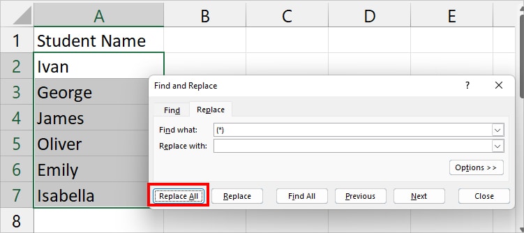
Use this method if the numbers are placed inside brackets. We will use Excel’s (*) Asterisk Wildcard characters to find them. Asterisks will find all numbers with brackets.
Note that in this approach, Find and Replace will directly eliminate numbers in the original data. So, keep a copy of the data if you think you’d need them later.
- On your spreadsheet, press down Ctrl + H for Find and Replace menu.
- Type in (*) in Find what.
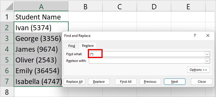
- Then, on Replace with, leave the field blank. Hit Replace All.
Using Text to Columns
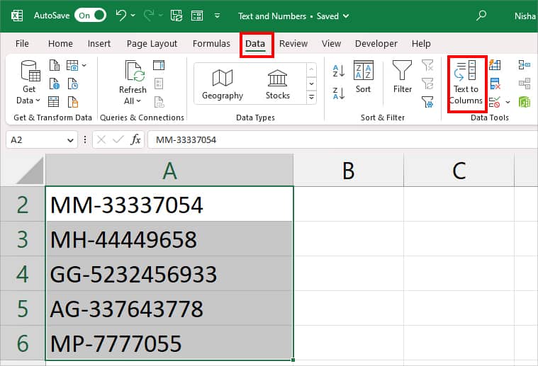
If you have numbers and texts separated by a delimiter, you can use the Text to Columns tool. With Text to Columns, you can split the text strings and numbers into two columns. Then, choose to import only the text columns in your sheet.
- Select your data. From Data Tab, click Text to Columns.
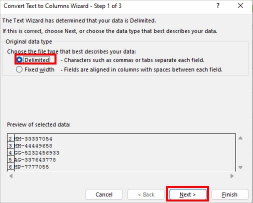
- On Step 1 of Convert Text to Columns Wizard, pick Delimited and click Next.
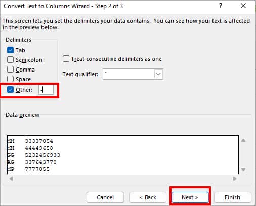
- On Step 2, tick Other option and enter – in the box. Hit Next.
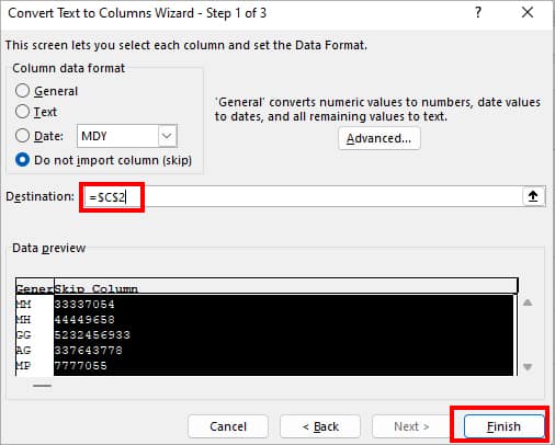
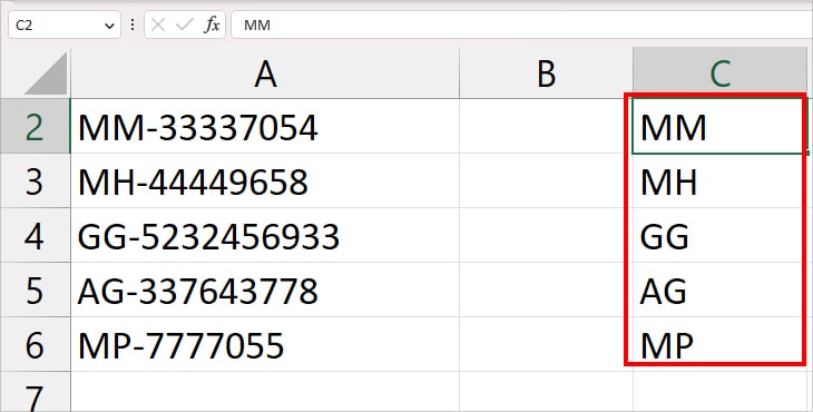
- On Step 3, select the Numbers column and choose Do not import column (skip).
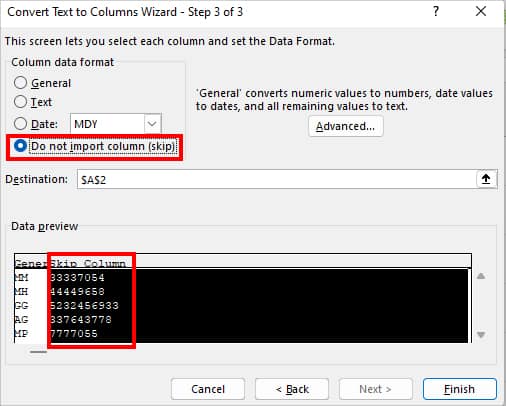
- Select a Destination to import Column and hit Finish.
- You won’t have numbers in texts anymore.
Using Formula
If you have combined values like 1A5B3C2D format, it is not possible to delete only numbers using the above method. In such cases, we will nest Excel’s different functions together like TEXTJOIN, IF, MID, SEQUENCE, LEN, etc.
Firstly, we will take a look into what each function means and its syntax in this table.
| Function | Syntax | Description |
| TEXTJOIN | TEXTJOIN(delimiter, ignore_empty, text 1, [text2],..) | Join texts of different cell ranges with a delimiter. For Example, 3rd North New York USA is in different Columns. Using TEXTJOIN, you can combine these text strings together to form 3rd North, New York, USA in one cell. |
| IF | IF(logical_test, value_if_true, [value_if_false]) | IF function tests the certain condition you pass down in a formula. Then, it returns two results. One value when the condition is TRUE and the other when the condition is FALSE. |
| ISERROR | ISERROR(value) | Tests if the value is an error or not. As a result, the function returns TRUE if there is an error like #VALUE! #NUM!, #SPILL!, #NAME?, #REF!, #NULL!, #CALC! in the value. Similarly, it returns FALSE if there are no errors. |
| MID | MID(text,start_num,num_chars) | Returns characters from the text strings. You can specify the starting position and total number of characters to extract. For Example, =MID(“Nisha”, 3,3) returns “sha”. |
| SEQUENCE | SEQUENCE(rows,[columns],[start],[step]) | SEQUENCE function returns the array of consecutive values. For Example, =SEQUENCE(2,3) returns an array of 123456 in two rows and 3 columns. |
| LEN | LEN(text) | Returns the total number of characters in a text string. For Example, =LEN(“Sunday”) returns 6. |
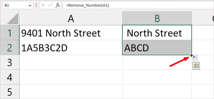
In the given case, let’s assume I have an address of 9401 North Street in cell A1. To delete numbers and keep only the texts I entered the following formula in the cell B1.
=TEXTJOIN("", TRUE, IF(ISERROR(MID(A1, SEQUENCE(LEN(A1)), 1)*1), MID(A1, SEQUENCE(LEN(A1)),1),""))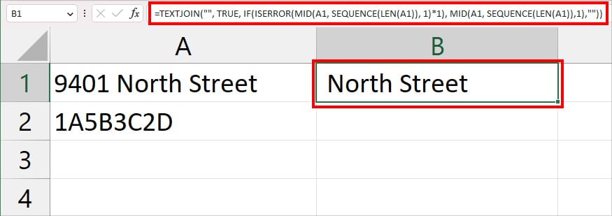
I know the formula looks extremely huge and intimidating. But, we will break down the formula and see how it works below.
- LEN(A1): Using the LEN function, we first returned 17 characters from the text “9401 North Street” in cell A1.
- SEQUENCE(LEN(A1)): SEQUENCE returns LEN(A1) rows in sequential order. For example, 1,2,3,4,5,6,7, till 17.
- MID(A1, SEQUENCE(LEN(A1)), 1)*1): Here, we’ve passed down the value of cell A1 “9401 North Street” as text in the MID function. Our character position is in SEQUENCE(LEN(A1)), and we will return only 1 character from the text. As a result, we got 9.
- ISERROR(MID(A1, SEQUENCE(LEN(A1)), 1)*1): It’ll check if there is an error in the Value which is 9. Since there isn’t any error, it returned FALSE.
- IF(ISERROR(MID(A1, SEQUENCE(LEN(A1)), 1)*1):
- Here, the IF function takes (ISERROR(MID(A1, SEQUENCE(LEN(A1)), 1)*1) as logical_test which is “FALSE”.
- If the value of MID(A1, SEQUENCE(LEN(A1)),1) is TRUE, it’ll return {“9”; “4”; “0”; “1”;” “;”“N”; “o”; “r” ; “t” ; “h”; “ ” “S”; “t” ; “r” ; “e” ; “e” ; “t”}.
- But, If the value of “” is FALSE, it’ll return only {“”; “”; “”; “”; “ ” “;”“N”; “o”; “r” ; “t” ; “h” ; “ ” ;“S”; “t” ; “r” ; “e” ; “e” ; “t”}
- In our case, since the value is FALSE, we got the latter answer.
- TEXTJOIN(“”, TRUE, IF(ISERROR(MID(A1, SEQUENCE(LEN(A1)), 1)*1), MID(A1, SEQUENCE(LEN(A1)),1),””)): Finally, TEXTJOIN joins all the characters inside the “” delimiter and returns North Street as a result.
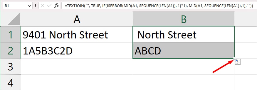
We even used the Flash-fill handle to copy down the formula to other cells.
Using VBA
If you find the above formula to delete numbers overwhelming, we also have a VBA code which is relatively easier to use. Here, we will first create our own function using Excel’s Visual Basics tool. Then, use the function to eliminate the numbers from text strings.
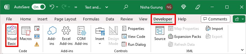
Before jumping into steps, check if you have the Developer tab in your Sheet. If there isn’t, you’d have to load them from the Options menu.
- Click Visual Basic from the Developer Tab.
- On Microsoft Visual Basic for Applications, click Insert > Module.
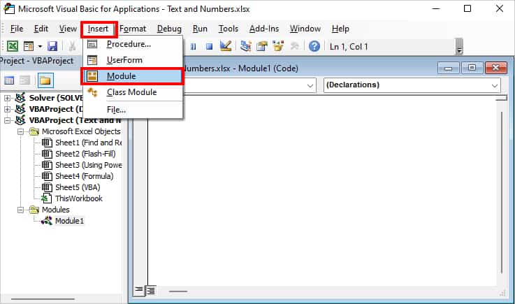
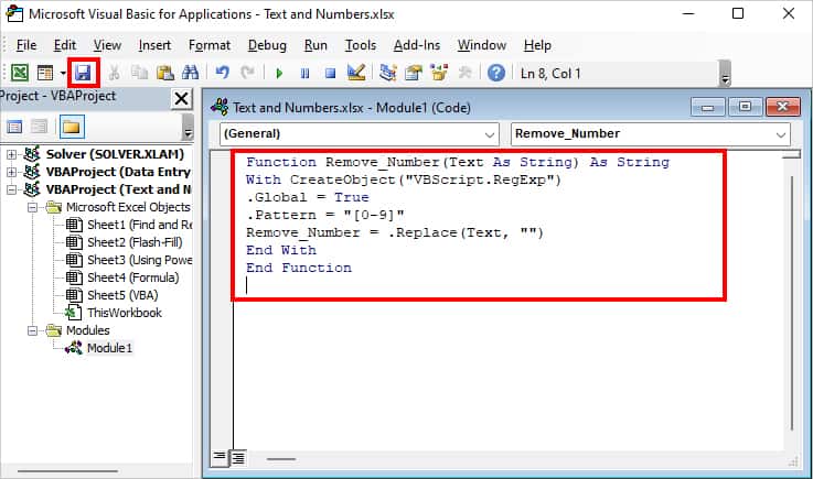
- Then, on the empty field, paste the given code.
Function Remove_Number(Text As String) As String
With CreateObject("VBScript.RegExp")
.Global = True
.Pattern = "[0-9]"
Remove_Number = .Replace(Text, "")
End With
End Function- Hit the Save button on the VBA window.
- Now, on a new cell, enter the formula as
=Remove_Number(A1).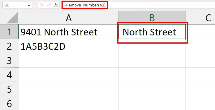
- Extend the flash-fill icon to fill the rest of the cells.