How to Remove Commas in Excel

As much as we like to work with clean/structured data only, it’s certainly not the case when importing data from external sources. Sometimes, unwanted characters like commas appear across all the text and we end up with texts like “Jackie, Reacher” instead of “Jackie Reacher” or similar.

Likewise, Excel uses commas as the thousands separator between the numbers (like 1,000) to make them more readable. However, commas in something like a student ID or employee ID are rather inappropriate or unnecessary. 

Nonetheless, we have compiled a list of built-in methods and functions to quickly get rid of them in various scenarios. Keep reading to learn more in detail.

Using the Find and Replace Tool

Usually, we use the Find and Replace tool to replace a particular text/character with a different one.

But, in this particular case, you can replace the comma with a blank character as well. 

1. Select the row, column, or cell range depending on where you want to replace the commas.
2. Then, press Ctrl + H.
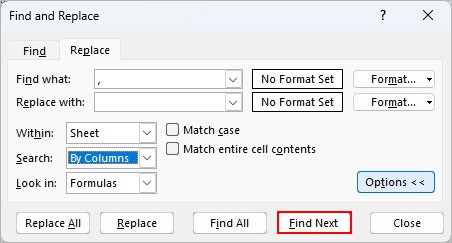
3. On the Find and Replace window, type , next to Find what field.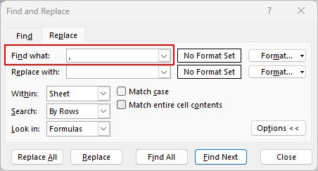
   
4. Next to Replace with field, enter another character you want instead of the comma Otherwise, leave it empty.
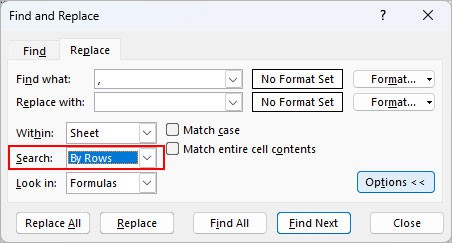
5. Choose one of the following options next to the Search field.
   • By Columns: To replace the comma in column (s)
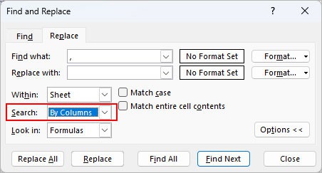
   • By Rows: To replace the comma in row (s)
6. Click Find Next to go through each cell where the comma will be replaced/ removed.
   
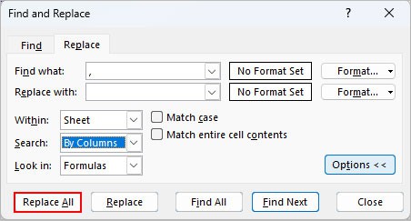
7. Click Replace All.
   

Using Power Query

The Power Query has a built-in feature similar to the Find and Replace tool, which can remove comma characters.

The Power Query also provides a similar feature like the Find and Replace tool to remove comma characters.

However, it provides additional options for several other data-cleaning operations like splitting parts of a text before or after a comma. Also, it allows an undo option to revert to the previous steps whenever required.

But, note that loading a huge dataset into Power Query can take some time. In that case, the Find and Replace function is a much quicker and more appropriate method.

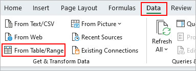
1. Select all cells containing your data.
2. Under the Data tab, click From Table/ Range. Look for it inside the Get & Transform Data.
   
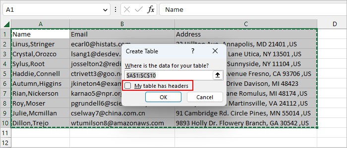
3. Enable the My table has headers if your data has headers.
   
4. On the Power Query Editor window, click the column header which contains the unwanted comma characters. To select multiple columns, press the Ctrl key while clicking them.
   
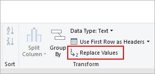
5. Then, select the Home tab and click Replace Values.
   
6. On the next prompt, type a comma character under the Value to Find section. Leave the Replace with field empty unless you want to replace the comma characters with others like spaces, dashes, etc.
   
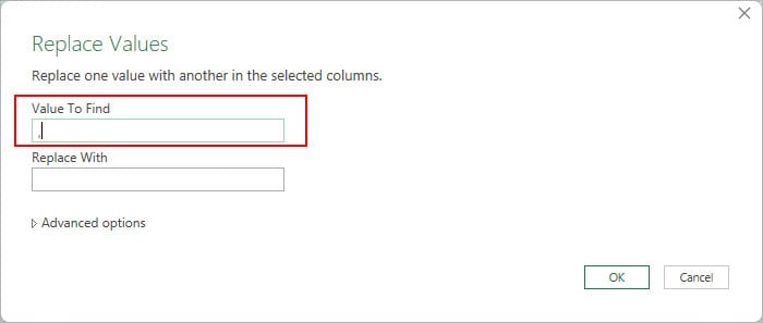
7. Click OK.
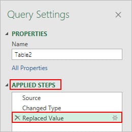
8. To undo a step, click the cross icon next to it under the Applied Steps section. You can find it at the right side.
   
9. When done, click Close & Load > Close & Load To.
   
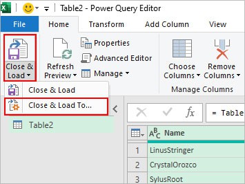
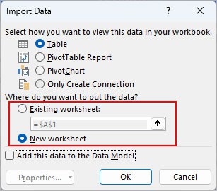
10. Choose the preferred destination to load the final output.
    

Using Custom Formatting

Whenever a number is using an accounting number format, Excel displays it with a comma, such as $1,000.00, €1,000.00, or similar. 

Also, Excel uses commas, by default, as the thousands separators resulting in a number like 1,000 or 1,000.00.

Whichever your case is, you can change and use custom formatting to avoid commas in numbers.

1. Select the cell (s) containing commas.
2. Press Ctrl + 1.
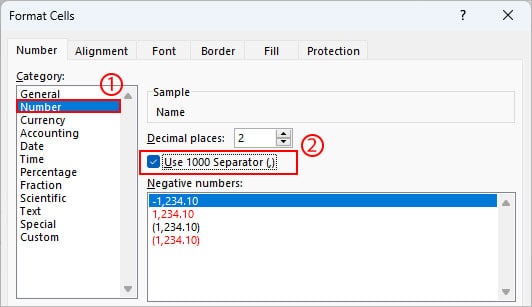
3. Select the Number tab.
4. Then, choose Number under the Category section.
5. Uncheck the Use 1000 Separator (,) checkbox.
   
6. Alternatively, select Custom under the Category section. Then, choose a different formatting under the Type section such as 0, #,##0, #,##0.00, etc.
   
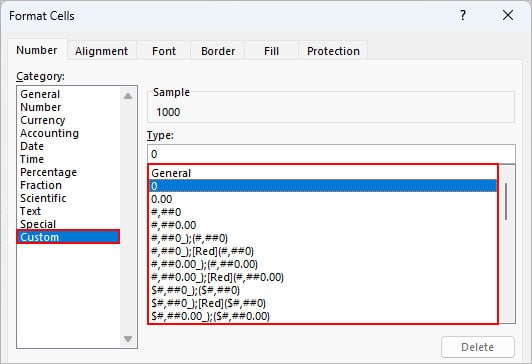
7. When done, click OK.

To change the comma character as the default thousands separator for the whole Excel application,

1. Open the Excel app.
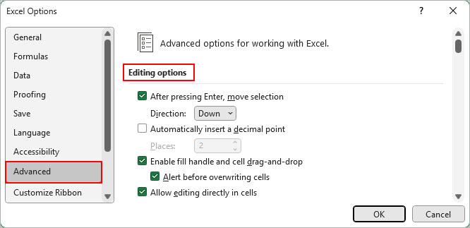
2. Then, select File > Options.
3. Next, select Advanced from the sidebar.
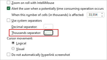
4. On the right pane, scroll down to the Editing options section.
   
5. Uncheck the Use system separators checkbox and replace the comma with the preferred thousands separator.
   

Using the SUBSTITUTE Function

As the name suggests, the Substitute function substitutes a particular value with another specified value. Using it, you can remove commas or replace them with other characters like a -,+, or any other character.

Syntax:=SUBSTITUTE(text, old_text, new_text)

Where,

• text: Cell or cell reference of the text containing a specific character like a comma
• old_text: The character you want to replace (comma in our case)
• new_text: A character that will replace the old_text character 

1. Create a helper column to hold values after removing commas.
2. Type the following formula under the new column. Replace A2:A10 with the cell range which contains the text values with commas in your dataset.
   =SUBSTITUTE(A2:A10,","," ")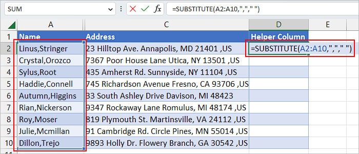
   
3. Press Enter.

Using Flash Fill

This method works particularly well given that texts with unwanted commas exist within the same column and follow the same pattern.

The good part is you don’t have to use any formula whatsoever. Also, it doesn’t necessarily remove every comma unless you want to. So, you can remove comma (s) existing at a particular position of a text value.

For instance, the text “Alexandria, VA 22304, USA” contains two commas. But, we only want to remove the first comma, giving us the result “Alexandria VA 22304, USA.”

1. Create a helper column to store text values without commas.
2. Manually type the text value without the comma (s) under the new column and press Enter.
3. Start typing the next text without the comma and as soon as Excel autocompletes other cells, press Enter.